A Model of Regulated Open Access Resource Use

More documents

Recommendations

Info

8 HOMANS AND WILEN equilibrium depicts the industry’s ‘‘choice’’ of a rent dissipating capacity, given the season length, and regulatory behavior is depicted as a choice of season length, given fishing capacity, the initial biomass, and the quota target established in the first stage. 2.3. Between-Season Dynamics and the Harest Quota Target The discussions above characterize an industry and regulator equilibrium during a single fishing season in which the initial biomass and hence quota are predetermined. If the quota is an equilibrium quota, the biomass will remain constant and the regulated open access fishery will be in a full steady state. If the biomass is changing, however, both the industry and regulator equilibrium curves will shift from season to season, since they are both functions of a changing X 0. 8 We can then think of the intersection of the two curves as determining a sequence of temporary equilibria, in which the industry and regulators attain successive withinseason equilibria, each associated with the existing biomass level each period. Over time we would observe the entire system moving through a sequence of temporary seasonal equilibria as the biomass approached its long run level. In order to close the model and describe this long run equilibrium, we thus need to specify the dynamic relationships which determine the evolution of biomass levels between seasons. The simplest way to specify this process is to utilize a hybrid Schaefer Beverton-Holt model in which within season dynamics are simply governed by Eqs. Ž. 1 and Ž. 2 above and between season dynamics are governed by a density dependent mechanism. That is, during the fishing season, total biomass is assumed to evolve to reflect the harvest rate, falling from its initial level X0 to XT by the end of the season. Then, between seasons, it is assumed that the net biological growth depends in some density dependent way on previous biomass. Let X 0, t1 be the biomass at the opening date of next year’s season and let XT , t and X0, t be the ending and beginning biomass levels this season, respectively. Here we are indexing seasons by t and denoting the beginning and ending dates of any particular season with 0 and T. Ž . 2 9 Assume that additions to the biomass can be defined as G X0, t aX0, t bX 0, t. Then between season dynamics can be represented by X0, t1 XT, t GŽ X0, t. XT, taX0, t bX0, 2 t. Ž 8. 8 In particular, the industry equilibrium function shifts up with increases in biomass. The regulatory equilibrium function may shift in or out, depending upon the form of the quota rule. It can be shown that the regulatory equation will shift out Ž in. if the regulatory rule is elastic Ž inelastic. with respect to biomass. Thus for a linear rule, the rectangular hyperbola will shift out as biomass increases if c is positive and in if c is negative. 9 Our use of the biomass growth function deserves some comment. Since halibut reach reproductive age in 7 to 8 years, it would be more realistic to employ an age-structured cohort model to capture biomass dynamics rather than a simple annual model. While the introduction of a cohort model may improve the accuracy of our representation of biomass dynamics and would be tractable for that purpose, it would introduce considerable analytical complexities into the complete model of season length and effort determination. Using a lumped parameter annual model for halibut has several precedents, see Cook 4 , Stollery 21 , and Conklin and Kolberg 5 .
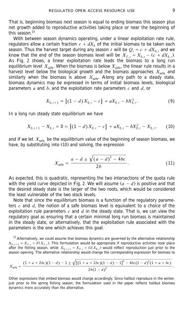
REGULATED OPEN ACCESS RESOURCE USE 9 That is, beginning biomass next season is equal to ending biomass this season plus net growth added to reproductive activities taking place or near the beginning of this season. 10 With between season dynamics operating, under a linear exploitation rate rule, regulators allow a certain fraction c dX0 of the initial biomass to be taken each season. Thus the harvest target during any season t will be Qt c dX0, t and we know that the end of the season biomass level will be X X Ž c dX . T , t 0, t 0, t . As Fig. 2 shows, a linear exploitation rate leads the biomass to a long run equilibrium level X safe. When the biomass is below X safe, the linear rule results in a harvest level below the biological growth and the biomass approaches Xsafe and similarly when the biomass is above X safe. Along any path to a steady state, biomass dynamics may be expressed in terms of initial biomass levels, biological parameters a and b, and the exploitation rate parameters c and d, or Ž . Ž . 2 X0, t1 1d X0, tc aX0, t bX 0, t. 9 In a long run steady state equilibrium we have Ž . Ž . 2 X0, t1 X0, t 0 1 d X0, t c aX0, t bX0, t X 0, t, 10 and if we let Xsafe be the equilibrium value of the beginning of season biomass, we have, by substituting into Ž 10. and solving, the expression ' 2 a d Ž a d. 4bc Xsafe . Ž 11. 2b As expected, this is quadratic, representing the two intersections of the quota rule with the yield curve depicted in Fig. 2. We will assume Ž a d. is positive and that the desired steady state is the larger of the two roots, which would be considered the least vulnerable of the two stock levels. Note that since the equilibrium biomass is a function of the regulatory parameters c and d, the notion of a safe biomass level is equivalent to a choice of the exploitation rule parameters c and d in the steady state. That is, we can view the regulatory goal as ensuring that a certain minimal long run biomass is maintained in the steady state, or alternatively, that the exploitation rule associated with the parameters is the one which achieves this goal. 10 Alternatively, we could assume that biomass dynamics are governed by the alternative relationship X X FŽ X . 0, t1 T , t T, t . This formulation would be appropriate if reproductive activities took place after the fishing season, while X X GŽ X . 0, t1 T , t 0, t would reflect reproduction just prior to the season opening. The alternative relationship would change the corresponding expression for biomass to Ž 1a2bc.Ž 1 d. 1 'Ž 1 a 2bc.Ž 1 d. 1 2 4bcŽ 1 d. 2 Ž 1 a bc. Xsafe . 2 2bŽ 1 d. Other expressions that embed biomass would change accordingly. Since halibut reproduce in the winter, just prior to the spring fishing season, the formulation used in the paper reflects halibut biomass dynamics more accurately than the alternative.
Page 1 and 2: Ž . JOURNAL OF ENVIRONMENTAL ECONO
Page 3 and 4: REGULATED OPEN ACCESS RESOURCE USE
Page 7: REGULATED OPEN ACCESS RESOURCE USE
Page 21: REGULATED OPEN ACCESS RESOURCE USE

A Model of Regulated Open Access Resource Use

You also want an ePaper? Increase the reach of your titles

Delete template?

Save as template?