A Model of Regulated Open Access Resource Use

More documents

Recommendations

Info

18 HOMANS AND WILEN rent dissipation in a manner similar to that first described by Gordon in 1954. In particular, with a Schaefer production function and with biomass dynamics within the season governed by harvesting mortality, undiscounted rents for any season are simply Rents PX0Ž 1 e qET . ET fE. Ž A1. This equation cannot be solved explicitly for capacity E as a function of other variables. Let JŽ E,T; X , P, q,, f. 0 describe the function obtained by setting rents in Ž A1. above equal to zero. Then we can use the implicit function theorem to get dE JT E PqX0 E qET . Ž A2 qET . dT J T PqX e f E 0 The denominator of this expression is the net value of marginal physical product of an additional unit of capacity. If capacity enters until rents are dissipated, the net value of average physical product will be zero. Since marginal product is less than average product, and since average product is zero, the denominator must be negative. The numerator of Ž A2. is the Ž negative of the. value of marginal physical product of an additional unit of season length. The sign of the numerator depends upon where in the domain of ET Ž . we are operating. As it turns out, in the relevant region, the value of marginal product is positive and hence the numerator is negative. This can be seen as follows. Let Ž ET . be variable profits associated with arbitrary levels of ET before fixed costs fE are subtracted, or PX 1 e qET ET. A3 0Ž . Ž . Note first that is strictly concave in E, T, and ET. In addition, the average variable profit function has a finite limit as E approaches zero, namely This leads to: lim Ž E. PqX T T . Ž A4. E0 PROPOSITION 1. A necessary and sufficient condition for positie leels of capacity is that the season length allowed by regulators T be larger than some T where 0 min f Tmin . Ž A5. PX q This can easily be seen by noting that capacity will enter only if average variable profits cover fixed entry costs. Since average variable profits are decreasing in E, there will be entry only if the first unit finds it profitable or if 0 lim Ž E. PqX T T f . Ž A6. E0 But this is true only if T is greater than T defined in Ž A5 . min . This defines a minimum season length below which no positive capacity is feasible. There is also a maximum season length T max, beyond which the industry would not voluntarily choose to fish. This can be seen by noting that the numerator of 0
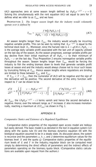
REGULATED OPEN ACCESS RESOURCE USE 19 Ž . qET A2 approaches zero at some season length defined by PqX0 e 0. Solving this simultaneously with the rent equation Ž A1. set equal to zero for T defines what we refer to as T and we have: max PROPOSITION 2. The longest season length that the industry would oluntarily operate oer is defined by f ln Ž PqX0. Tmax . Ž A7. PqX 1 ln Ž PqX . Ž . 0 0 At season lengths longer than T max, the industry would actually be incurring negative variable profits. This can be seen by noting that X0 e qET is equal to the terminal stock level X . Moreover, since the harvest rate is h qEXŽ. T t , PqXT is the average daily variable profit associated with the last unit of capacity utilized on the last day of the season. As the season progresses, average variable profits per day decline from their initial maximum of of PqX to their minimum of 0 PqXT on the last day. Thus Proposition 2 ensures nonnegative variable profits throughout the season. Season lengths larger than T would be forcing the industry to fish the ending biomass down to levels that generate variable profit losses at season end and the industry would always choose not to incur such losses by truncating fishing at T max. Hence season lengths where regulations are binding are limited to those between Tmin and T max. If T T T , then the numerator of Ž A2. will be negative and the sign of min max the derivative will be positive. The second derivative of the entry function with respect to T can be shown to be 2 qET 2 2 2 qET 0 0 dE PqX e f Pq EX e E 2 . Ž A8 2 qET 3 . dT T Ž PqX e . f qET 0 T PqX e f max Ž 0 . Ž qET At T , the PqX e . max 0 terms vanish and hence the second derivative is negative. Hence, over the relevant range, as T increases E also increases monotonically, reaching a maximum at ET Ž . as shown in Fig. 1. max APPENDIX B Comparatie Statics and Existence of a Regulated Equilibrium Comparative statics properties of the regulated open access model are tedious but easily derived. The basic model is as denoted in the text in equation system Ž 12. along with the quota rule Ž. 5 and the biomass dynamics equation Ž. 8 with the biological equation assumed to be in a steady state. As discussed above, the system is recursive and the parameters a, b, c, and d determine equilibrium values for the biomass level X and the quota Q. Comparative statics properties of the equilibrium levels of E and T in the industryregulator block can be computed most simply by determining the direct effects of parameters and the indirect effects of parameters operating on the biomassquota block. ŽComparative statics calculations are available upon request from the authors..
Page 1 and 2: Ž . JOURNAL OF ENVIRONMENTAL ECONO
Page 3 and 4: REGULATED OPEN ACCESS RESOURCE USE
Page 17: REGULATED OPEN ACCESS RESOURCE USE
Page 21: REGULATED OPEN ACCESS RESOURCE USE

A Model of Regulated Open Access Resource Use

You also want an ePaper? Increase the reach of your titles

Delete template?

Save as template?