the equivalence of chebyshev's inequality to the hermite-hadamard ...

Dedicated to Professor Gheorghe Bucur
on the occasion of his 70th birthday
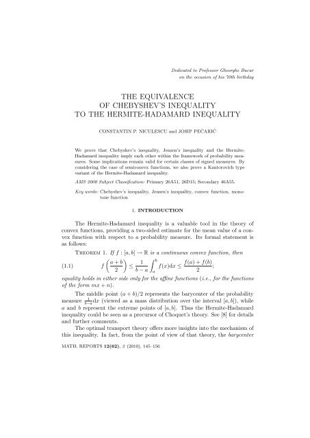
THE EQUIVALENCE
OF CHEBYSHEV’S INEQUALITY
TO THE HERMITE-HADAMARD INEQUALITY
CONSTANTIN P. NICULESCU and JOSIP PEČARIĆ
We prove that Chebyshev’s inequality, Jensen’s inequality and the Hermite-
Hadamard inequality imply each other within the framework of probability measures.
Some implications remain valid for certain classes of signed measures. By
considering the case of semiconvex functions, we also prove a Kantorovich type
variant of the Hermite-Hadamard inequality.
AMS 2000 Subject Classification: Primary 26A51, 26D15; Secondary 46A55.
Key words: Chebyshev’s inequality, Jensen’s inequality, convex function, monotone
function
1. INTRODUCTION
The Hermite-Hadamard inequality is a valuable tool in the theory of
convex functions, providing a two-sided estimate for the mean value of a convex
function with respect to a probability measure. Its formal statement is
as follows:
Theorem 1. If f : [a, b] → R is a continuous convex function, then
( ) a + b
(1.1) f ≤ 1 ∫ b
f(a) + f(b)
f(x)dx ≤ ;
2 b − a
2
a
equality holds in either side only for the affine functions (i.e., for the functions
of the form mx + n).
The middle point (a + b)/2 represents the barycenter of the probability
1
measure
b−adx (viewed as a mass distribution over the interval [a, b]), while
a and b represent the extreme points of [a, b]. Thus the Hermite-Hadamard
inequality could be seen as a precursor of Choquet’s theory. See [8] for details
and further comments.
The optimal transport theory offers more insights into the mechanism of
this inequality. In fact, from the point of view of that theory, the barycenter
MATH. REPORTS 12(62), 2 (2010), 145–156

146 Constantin P. Niculescu and Josip Pečarić 2
of a mass distribution on [a, b], represented by a Borel probability measure µ,
is the unique minimizer b µ of the transportation cost,
C(y) = 1 2
∫ b
a
|x − y| 2 dµ(x),
associated to the cost function c(x, y) = 1 2 |x − y|2 . See [11]. The transportation
cost being uniformly convex, it attains its minimum at the unique root
of its derivative, so that
b µ =
∫ b
a
xdµ(x).
It is useful to formulate the Hermite-Hadamard inequality (1.1) in the
context of semiconvex functions and arbitrary mass distributions.
Definition 1. A function f : [a, b] → R is called semiconvex (of rate k) if
the function f + k 2 | · |2 is convex for some real constant k, that is,
f((1 − λ)x + λy) ≤ (1 − λ)f(x) + λf(y) + k λ(1 − λ) |x − y|2
2
for all x, y ∈ [a, b] and all λ ∈ [0, 1].
For example, every twice differentiable function f such that f ′′ +k ≥ 0 is
semiconvex of rate k. A semiconvex function of negative rate is usually known
as an uniformly convex function.
A useful remark is that a function f is semiconvex of rate k if and only
if for some point x 0 ∈ [a, b] (equivalently, for any point x 0 ) the function
h(x) = f(x) + k 2 |x − x 0| 2
is convex.
Based on Choquet’s theory we can state the following generalization of
the Hermite-Hadamard inequality in the context of semiconvex functions:
Theorem 2. If µ is a Borel probability measure on an interval [a, b],
then for every semiconvex function f : [a, b] → R of rate k we have
(1.2)
f(b µ ) ≤
∫ b
a
f(x)dµ(x) + k 2
∫ b
a
|x − b µ | 2 dµ(x)
≤ b − b µ
b − a · f(a) + b µ − a
b − a · f(b) + k 2 (b µ − a)(b − b µ ).
The term (b µ −a)(b−b µ ) represents the transportation cost of the mass δ bµ
to b−bµ
b−a δ a + bµ−a
b−a δ b. This proves to be more expansive than the transportation
cost of µ to δ bµ (a fact which follows from the right hand side inequality in

3 Chebyshev’s inequality and the Hermite-Hadamard inequality 147
Theorem 2, when applied to the function f(x) = |x − b µ | 2 and k = 0). The
difference of the two costs
(1.3) D(µ) = (b − b µ ) (b µ − a) −
∫ b
a
|x − b µ | 2 dµ(x),
is thus nonnegative and it reflects both the geometry of the domain and the
mass distribution on it.
The aim of this paper is to discuss the connection of the Hermite-
Hadamard inequality to another classical result, Chebyshev’s inequality.
Theorem 3 (Chebyshev’s inequality). If f, g : [a, b] → R are two monotonic
functions of the same monotonicity, then
∫
1 b
( ∫ 1 b
) ( ∫ 1 b
)
f(x)g(x)dx ≥
f(x)dx
g(x)dx .
b − a
b − a
b − a
a
If f and g are of opposite monotonicity, then the above inequality works in the
reverse way.
The proof of Theorem 3 is a direct consequence of the property of positivity
of the integral. The basic remark is the inequality
(f(x) − f(y)) (g(x) − g(y)) ≥ 0
a
a
for all x, y ∈ [a, b],
which is integrated with respect to x and y.
No argument of such simplicity is known for Theorem 1.
Remark 1. In the statement of Theorem 3, the interval [a, b] can be
1
replaced by any interval I, and the normalized Lebesgue measure
b−adx can
be replaced by any Borel probability measure on the interval I. The argument
remains the same!
Surprisingly, Theorem 1 can be derived from Theorem 3 (and vice-versa).
This is shown in the next section. When the normalized Lebesgue measure is
replaced by an arbitrary Borel probability measure (still defined on a compact
interval), the left hand side inequality in Theorem 2 is equivalent to Jensen’s
inequality (for k = 0), which in turn is equivalent to Chebyshev’s inequality.
Steffensen’s extension of Jensen’s inequality (see [8], p. 33), started the
important subject of generalizing the classical inequalities to the framework
of signed Borel measures.
Based on previous work done (independently) by T. Popoviciu and A.M.
Fink, the first named author was able to provide a characterization of those
signed Borel measures for which Jensen’s inequality remains valid in full generality.
See [8], Section 4.1, for details. A characterization of the signed Borel
measures defined on a compact interval for which both sides of the Hermite-
Hadamard inequality still work can be found in [4]. A tantalizing problem

148 Constantin P. Niculescu and Josip Pečarić 4
is the characterization of such measures in the case of several variables. A
particular result in this direction is presented in [5].
The problem of characterizing the signed Borel measures for which Chebyshev’s
inequality remains valid was solved by Fink and Jodeit Jr. [3]. See also
[6], Ch. IX. At about the same time Pečarić [9] has provided an elegant (partial)
solution based on an identity describing the precision in Chebyshev’s
inequality. His approach is put here in full generality, being accompanied by
an analogue of the Grüss inequality. See Theorem 5 below. As a consequence
we are able to derive the Jensen-Steffensen inequality as well as an estimate
of its precision.
The paper ends with a generalization of Kantorovich’s inequality within
the framework of signed measures.
2. PROOF OF THEOREM 2
We start by noticing that Theorem 3 is strong enough to yield the classical
inequality of Jensen.
Theorem 4 (Jensen’s inequality). If (X, Σ, µ) is a finite measure space,
ϕ : X → R is a µ-integrable function and h is a continuous convex function
defined on an interval I containing the range of ϕ, then
(2.1) h
( 1
µ(X)
∫
X
)
ϕ(x)dµ(x)
≤ 1
µ(X)
∫
X
h (ϕ(x))dµ(x).
Proof. If h : I → R is a convex function, and c ∈ int I is kept fixed, then
the function
h(x) − h(c)
x →
x − c
is nondecreasing on I\{c}. Let ν be a finite positive Borel measure on I
with barycenter
b ν = 1 ∫
xdν(x).
ν(I) I
Clearly, b ν ∈ I (since otherwise b ν − x or x − b ν will provide an example of
strictly positive function whose integral with respect to ν is 0). According to
Chebyshev’s inequality, if b ν ∈ int I, then
∫
1 h(x) − h(b ν )
(x − b ν )dν(x) ≥
≥ 1 ∫
ν(I) I
ν(I) I x − b ν
h(x) − h(b ν )
dν(x) ·
x − b ν
1
ν(I)
∫
I
(x − b ν ) dν(x) = 0,

5 Chebyshev’s inequality and the Hermite-Hadamard inequality 149
which yields
(2.2) h(b ν ) ≤
1
ν([a, b])
∫ b
a
h(x)dν(x).
Notice that the last inequality also works when b ν is an endpoint of I (because
in that case ν = δ bν ).
Using the technique of pushing-forward measures, we can infer from (2.2)
the general statement of the Jensen inequality. In fact, if µ is a positive Borel
measure on X and ϕ : X → I is a µ-integrable map, then the push-forward
measure ν = ϕ#µ is given by the formula ν(A) = µ(ϕ −1 (A)) and its barycenter
is
According to (2.2),
h(ϕ) ≤ 1
ν(I)
ϕ = 1
µ(X)
∫
I
∫
X
ϕ(x)dµ(x).
h(t)dν(t) = 1 ∫
h(ϕ(x))dµ(x)
µ(X) X
for all continuous convex functions h : I → R, which ends the proof of Theorem
4. □
It is clear that the inequality of Jensen implies in turn the positivity property
of integral (and thus all are equivalent to the inequality of Chebyshev).
The inequality of Jensen and the inequality of Chebyshev are also dual
each other. See [8], Section 1.8.
Coming back to the proof of Theorem 2, we will notice that the left hand
side inequality in (2) is a consequence of the inequality of Jensen (2.1), applied
to ϕ the identity of [a, b], and to the convex function h(x) = f(x)+ k 2 |x − b µ| 2 .
The right hand side inequality in (2) can be obtained in a similar manner,
as a consequence of the following result:
Lemma 1. For every convex function h : [a, b] → R and every Borel
probability measure µ on [a, b],
(2.3)
∫ b
a
h(x)dµ(x) ≤ b − b µ
b − a · h(a) + b µ − a
b − a · h(b).
Proof. Formally, this is a special case of an important theorem due to
Choquet. See [8], Section 4.4, for details. A more direct argument is in order.
If µ = ∑ n
i=1 λ iδ xi is a discrete probability measure, then its barycenter
is b µ = ∑ n
i=1 λ ix i and (2.3) takes the form
∑
n∑
b − n n∑
λ i x i λ i x i − a
i=1
i=1
(2.4)
λ i h(x i ) ≤
h(a) +
h(b).
b − a
b − a
i=1

150 Constantin P. Niculescu and Josip Pečarić 6
This inequality follows directly from the property of h of being convex. In fact,
which yields
x i = b − x i
b − a · a + x i − a
b − a · b
h(x i ) ≤ b − x i
b − a · h(a) + x i − a
b − a · h(b).
Multiplying both sides by λ i and then summing over i we arrive at (2.4).
The general case of (2.3) is now a consequence of the following approximation
argument: every Borel probability measure λ on a compact Hausdorff space is
the pointwise limit of a net of discrete probability measures, each having the
same barycenter as λ (see [8], Lemma 4.1.10, p. 183). □
When dµ = 1
b−adx is the normalized Lebesgue measure on [a, b], then
b µ = (a+b)/2 and we can derive the inequality (2.3) directly from Chebyshev’s
inequality. In fact,
∫
1 b
(
x − a + b )
h ′ (x)dx ≥
b − a
2
and
≥ 1
b − a
= 1
b − a
∫ b
a
∫ b
a
a
(
x − a + b
2
∫ b
1
b − a a
((
x − a + b
2
=
h(a) + h(b)
2
)
dx ·
(
x − a + b
2
)
h(x)
− 1
b − a
1
b − a
∫ b
a
)
h ′ (x)dx =
) ′
dx − 1
b − a
∫ b
a
h(x)dx.
h ′ (x)dx = 0
∫ b
3. THE CASE OF SIGNED MEASURES
a
h(x)dx =
Is is well known that the integral inequalities with respect to signed measures
are considerably more involving because the positivity property of the
integral does not work in that context. Notably, both Chebyshev’s inequality
and Jensen’s inequality admit extensions that work for certain signed measures.
The case of Chebyshev’s inequality is discussed by J. Pečarić in [9], Theorem
1, in the case of Stieltjes measures associated to absolutely continuous
functions. His basic argument is an identity whose validity can be established
under less restrictive hypotheses:

7 Chebyshev’s inequality and the Hermite-Hadamard inequality 151
Lemma 2. Suppose that p, f, g : [a, b] → R are functions of bounded
variation and f and g are also continuous. Then
(3.1)
=
∫ b
a
(p(b) − p(a))
∫ b
a
f(x)g(x)dp(x) −
(∫ x
)
p ∗ (x) p ∗ (t)dg(t) df(x) +
a
∫ b
a
∫ b
where p ∗ (x) = p(b) − p(x) and p ∗ (x) = p(x) − p(a).
a
f(x)dp(x)
∫ b
a
g(x)dp(x)
(∫ b
)
p ∗ (x) p ∗ (t)dg(t) df(x),
Proof. We start by noticing that the indefinite integral ∫ x
a
h(t)dp(t) of
any continuous function h has bounded variation and verifies the formula
∫ b
(∫ x
) ∫ b
f(x)d h(t)dp(t) = f(x)h(x)dp(x).
Thus for
h(t) =
∫ b
a
a
a
g(s)dp(s) − (p(b) − p(a)) g(t) =
a
∫ b
the formula of integration by parts leads us to the identity
∫ b
(∫ x
)
h(t)dp(t) df(x) =
= (p(b) − p(a))
On the other hand,
∫ x
a
a
∫ b
h(t)dp(t) = (p(x) − p(a))
(∫ x
=(p(x) − p(a)) g(t)dp(t) +
so that
=
∫ b
a
a
a
= −p ∗ (x)
= p ∗ (x)
(p(b) − p(a))
a
f(x)g(x)dp(x) −
∫ x
a
∫ x
∫ b
a
a
∫ b
a
∫ b
x
∫ b
a
a
x
f(x)dp(x)
(g(s) − g(t)) dp(s),
∫ b
g(t)dp(t) − (p(b) − p(a))
a
g(x)dp(x).
∫ x
)
g(s)dp(s) − (p(b) − p(a))
g(t)dp ∗ (t) − p ∗ (x)
∫ b
(∫ b
p ∗ (t)dg(t) + p ∗ (x)
f(x)g(x)dp(x) −
(∫ x
)
p ∗ (x) p ∗ (t)dg(t) df(x) +
a
∫ b
a
∫ b
a
x
x
g(t)dp ∗ (t) =
)
p ∗ (t)dg(t) ,
f(x)dp(x)
∫ b
a
a
∫ x
g(t)dp(t) =
a
g(x)dp(x)
g(t)dp(t)=
(∫ b
)
p ∗ (x) p ∗ (t)dg(t) df(x).
x
□

152 Constantin P. Niculescu and Josip Pečarić 8
An immediate consequence of Lemma 2 is the following stronger form of
Chebyshev’s inequality:
Theorem 5. Suppose that p : [a, b] → R is a function of bounded variation
such that
(3.2) p(b) > p(a) and p(a) ≤ p(x) ≤ p(b) for all x.
Then for every pair of continuous functions f, g : [a, b] → R which are monotonic
in the same sense, the Chebyshev functional
(
−
1
T (f, g; p) =
p(b) − p(a)
∫ b
) (
f(x)dp(x)
1
p(b) − p(a)
is bounded from above by
1
p(b)−p(a)
∫ b
a
a
∫ b
a
f(x)g(x)dp(x) −
1
p(b) − p(a)
∫ b
a
)
g(x)dp(x) ,
max{p ∗ 1
(x), p ∗ (x)}df(x) ·
max{p ∗ (x), p ∗ (x)}dg(x)
p(b)−p(a) a
≤ (f(b) − f(a))(g(b) − g(a)),
and is bounded from below by
1
p(b)−p(a)
∫ b
a
min{p ∗ 1
(x), p ∗ (x)}df(x)·
p(b)−p(a)
∫ b
a
∫ b
min{p ∗ (x), p ∗ (x)}dg(x)≥0.
Proof. In fact, we may assume that both functions f and g are nondecreasing
(changing f and g by −f and −g if necessary). Since the integral of a
nonnegative function with respect to a nondecreasing function is nonnegative,
we have
∫ b
a
(∫ x
p ∗ (x)
≥
+
∫ b
a
∫ b
=
a
∫ b
a
)
p ∗ (t)dg(t) df(x) +
∫ b
a
(∫ b
)
p ∗ (x) p ∗ (t)dg(t) df(x) ≥
x
)
df(x)+
(∫ x
min {p ∗ (x), p ∗ (x)} min {p ∗ (t), p ∗ (t)} dg(t)
(∫ b
min {p ∗ (x), p ∗ (x)}
a
min {p ∗ (x), p ∗ (x)} df(x) ·
a
x
)
min {p ∗ (t), p ∗ (t)} dg(t) df(x) =
∫ b
a
min {p ∗ (x), p ∗ (x)} dg(x)

9 Chebyshev’s inequality and the Hermite-Hadamard inequality 153
and
∫ b
a
≤
(∫ x
p ∗ (x)
∫ b
a
a
)
p ∗ (t)dg(t) df(x) +
max {p ∗ (x), p ∗ (x)} df(x) ·
∫ b
a
∫ b
a
(∫ b
)
p ∗ (x) p ∗ (t)dg(t) df(x) ≤
x
max {p ∗ (x), p ∗ (x)} dg(x).
Remark 2. As was noticed by Pečarić [9], very efficient bounds can be
indicated in the framework of C 1 -differentiability of f and g. For example, if
f and g are monotonic in the same sense, and |f ′ | ≤ α and |g ′ | ≤ β (for some
positive constants α and β), then
T (f, g; p) ≤ αβT (x − a, x − a; p).
The necessity of the condition (3.2) for the validity of Chebyshev’s inequality
is discussed in [3].
Theorem 5 yields the following improvement on the Jensen-Steffensen
inequality:
Theorem 6. Suppose that p : [a, b] → R is a function with bounded
variation such that p(b) > p(a) and p(a) ≤ p(x) ≤ p(b) for all x. Then for
every continuous and strictly monotonic function ϕ : [a, b] → R and for every
continuous convex function h defined on an interval I that contains the image
of ϕ, the inequality
holds. Here
∫ b
1
0 ≤
h (ϕ(x))dp(x) − h (b p ) ≤
p(b) − p(a) a
( h(ϕ(b)) − h(bp )
≤
− h(ϕ(a)) − h(b )
p)
(ϕ(b) − ϕ(a)) .
ϕ(b) − b p ϕ(a) − b p
b p =
1
p(b) − p(a)
∫ b
a
ϕ(x)dp(x)
represents the barycenter of the push-forward measure ϕ#dp.
Proof. Using an approximation argument we may restrict ourselves to
the case where h is differentiable. The functions ϕ(x) and h(ϕ(x))−h(bp)
ϕ(x)−b p
being
monotonic in the same sense, Theorem 5 applies and it gives us
≥
1
p(b) − p(a)
1
p(b) − p(a)
∫ b
a
∫ b
a
h(ϕ(x)) − h(b p )
(ϕ(x) − b p )dp(x) ≥
ϕ(x) − b p
h(ϕ(x)) − h(b p )
1
dp(x) ·
ϕ(x) − b p p(b) − p(a)
∫ b
a
□
(ϕ(x) − b p )dp(x) = 0.

154 Constantin P. Niculescu and Josip Pečarić 10
Thus
h(b p ) ≤
1
p(b) − p(a)
∫ b
a
h (ϕ(x))dp(x).
The proof ends by taking into account the discrepancy in Chebyshev’s
inequality (provided by Theorem 5). □
Remark 3. According to Lemma 2,
=
1
p(b) − p(a)
∫
1
b
(p(b) − p(a)) 2
∫
1
b
+
(p(b) − p(a)) 2
a
a
∫ b
(
p ∗ (x)
(
p ∗ (x)
a
∫ x
h (ϕ(x))dp(x) − h (b p ) =
a
∫ b
x
) ( )
h(ϕ(x)) − h(bp )
p ∗ (t)dϕ(t) d
+
ϕ(x) − b p
)
p ∗ (t)dϕ(t) d
( )
h(ϕ(x)) − h(bp )
,
ϕ(x) − b p
and this fact may be used to derive better bounds for the discrepancy in
Chebyshev’s inequality.
The fact that Theorem 1.2 works outside the framework of positive Borel
measures is discussed in [4] (under the nonrestrictive assumption that k = 0).
Let us call a real Borel measure µ on [a, b] , with µ ([a, b]) > 0, a Hermite-
Hadamard measure if for every convex function f : [a, b] → R the following
two inequalities hold true,
(LHH)
and
(RHH)
1
µ([a, b])
f(b µ ) ≤
∫ b
a
1
µ([a, b])
∫ b
a
f(x)dµ(x)
f(x)dµ(x) ≤ b − b µ
b − a · f(a) + b µ − a
b − a · f(b),
where b µ = 1 ∫ b
µ([a,b]) a xdµ(x).
According to [4], the measure (x 2 + a)dx verifies (LHH) (respectively
(RHH)) for all convex functions defined on the interval [−1, 1] if and and only
if a ≥ −1/3 (respectively a ≥ −1/6).
As a consequence, we can exhibit examples of functions of bounded variation
as in Theorem 5, which do not give rise to Hermite-Hadamard measures.
So is the function p(x) = (x 3 − 3x 4
), for x ∈ [−1, 1], which clearly verifies the
condition p(cos x) = 1 4
cos 3x ∈ [p(−1), p(1)]. However, the associated measure
dµ = 3(x 2 − 1 4
)dx does not verify (RHH) for all convex functions defined on
the interval [−1, 1].

11 Chebyshev’s inequality and the Hermite-Hadamard inequality 155
4. AN APPLICATION TO KANTOROVICH’S INEQUALITY
We start with the following variant of Theorem 2.
Theorem 7. Suppose that µ is a Hermite-Hadamard measure on [a, b],
with b µ > 0. Then for every k-convex function f : [a, b] → R such that
f(a) > f(b),
∫ b
∫ b
f(b µ ) − k |x − b µ | 2 dµ(x) ≤ f(x)dµ(x) ≤
2 a
a
[
bf(a) − af(b) +
1
2
≤
k(b − a)D(µ)] 2
,
4b µ (b − a) (f(a) − f(b))
where D(µ) is given by the formula (1.3).
Proof. The left hand side inequality is equivalent to the left hand side
inequality in Theorem 2. As concerns the right hand side inequality, it suffices
to consider the case where ∫ b
a
f(x)dµ(x) > 0. In this case, we make again an
appeal to Theorem 2 in order to infer that
This yields
(b − a)
∫ b
a
f(x)dµ(x) + (b − a) k 2
∫ b
a
|x − b µ | 2 dµ(x) ≤
≤ bf(a) − af(b) + (f(b) − f(a))b µ + k 2 (b − a) (b − b µ) (b µ − a) .
bf(a) − af(b) + k 2 (b − a) [(b − b µ ) (b µ − a) −
≥ (b − a)
and the proof is done.
∫ b
a
[
≥ 2 b µ (b − a) (f(a) − f(b))
□
∫ b
f(x)dµ(x) + (f(a) − f(b))b µ ≥
∫ b
a
a
]
|x − b µ | 2 dµ(x) ≥
f(x)dµ(x)] 1/2
,
Corollary 1. If f : [a, b] → R is a convex function such that f(a) >
f(b), and µ is a Hermite-Hadamard measure on [a, b] with b µ > 0, then
∫ b
(bf(a) − af(b)) 2
f(x)dµ(x) ≤
a
4b µ (b − a) (f(a) − f(b)) .
In the discrete case, when µ is a Borel probability measure of the form
µ = ∑ n
i=1 λ iδ xi , the result of Corollary 1 reads as
( n∑
) ( n∑
λ i x i λ i f(x i )
i=1
i=1
)
≤
(bf(a) − af(b)) 2
4 (b − a) (f(a) − f(b)) .

156 Constantin P. Niculescu and Josip Pečarić 12
If we apply this remark to the convex function f(x) = 1/x for x ∈ [m, M]
(where 0 < m < M), we recover a classical inequality due to Kantorovich:
( n∑
) ( n∑
)
λ i (M + m)2
λ i x i ≤
x
i=1
i=1 i 4Mm ,
for all x 1 , . . . , x n ∈ [m, M] and all λ 1 , . . . , λ n ∈ [0, 1] with ∑ n
i=1 λ i = 1. See [1].
However, our approach yields a bit more. Precisely, the Kantorovich
inequality still works for those Hermite-Hadamard measures ∑ n
i=1 λ iδ xi (on
[m, M]) such that ∑ n
i=1 λ ix i ∈ [m, M].
REFERENCES
[1] E.F. Beckenbach and R. Bellman, Inequalities, 2nd Ed., Springer-Verlag, Berlin, 1983.
[2] A.M. Fink, A best possible Hadamard Inequality. Math. Inequal. Appl. 1 (1998), 223–
230.
[3] A.M. Fink and M. Jodeit Jr., On Chebyšhev’s other inequality. In: Inequalities in Statistics
and Probability, IMS Lecture Notes Monograph Series, Vol. 5, 1984, 115–120.
[4] A. Florea and C.P. Niculescu, A Hermite-Hadamard inequality for convex-concave symmetric
functions. Bull. Soc. Sci. Math. Roum. 50(98) (2007), 2, 149–156.
[5] M. Mihăilescu and C.P. Niculescu, An extension of the Hermite-Hadamard inequality
through subharmonic functions. Glasgow Math. J. 49 (2007), 509–514.
[6] D.S. Mitrinović, J.E. Pečarić and A.M. Fink, Classical and New Inequalities in Analysis.
Kluwer, Dordrecht, 1993.
[7] C.P. Niculescu, An extension of Chebyshev’s inequality and its connection with Jensen’s
inequality. Journal of Inequalities and Applications 6 (2001), 451–462.
[8] C.P. Niculescu and L.-E. Persson, Convex Functions and their Applications. A Contemporary
Approach. CMS Books in Mathematics, Vol. 23, Springer-Verlag, New York,
2006.
[9] J.E. Pečarić, On the Ostrowski generalization of Čebyšev’s inequality. J. Math. Anal.
Appl. 102 (1984), 479–484.
[10] J.E. Pečarić, F. Proschan and Y.C. Tong, Convex functions, Partial Orderings and
Statistical Applications. Academic Press, New York, 1992.
[11] C. Villani, Optimal Transport. Old and New. Springer-Verlag, 2009.
Received 19 July 2009
University of Craiova
Department of Mathematics
200585 Craiova, Romania
cniculescu47@yahoo.com
and
University of Zagreb
Faculty of Textile Technology
Pierottijeva 6
10000 Zagreb, Croatia
pecaric@mahazu.hazu.hr