chapter 8. electron beams: physical and clinical aspects - IRSN

Review of Radiation Oncology Physics: A Handbook for Teachers and Students
CHAPTER 8.
ELECTRON BEAMS: PHYSICAL AND CLINICAL ASPECTS
WYNAND STRYDOM
Department of Medical Physics
Medical University of South Africa
Pretoria, South Africa
WILLIAM PARKER
Department of Medical Physics
McGill University Health Centre
Montréal, Québec, Canada
MARINA OLIVARES
Department of Medical Physics
McGill University Health Centre
Montréal, Québec, Canada
8.1. CENTRAL AXIS DEPTH DOSE DISTRIBUTIONS IN WATER
Megavoltage electron beams represent an important treatment modality in modern
radiotherapy, often providing a unique option in treatment of superficial tumours (less than 5
cm deep). Electrons have been used in radiotherapy since the early 1950s, first produced by
betatrons and then by linear accelerators (linacs). Modern high-energy linacs typically
provide, in addition to two megavoltage photon energies, several electron beam energies in
the range from 4 MeV to 22 MeV.
8.1.1 General shape of depth dose curve
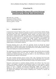
The general shape of the central axis depth dose curve for electron beams differs from that of
photon beams, as seen in Fig. 8.1. that shows depth doses for various electron beam energies
in part (a) and depth doses for 6 MV and 15 MV x-ray beams in part (b). Typically, the
electron beam central axis depth dose curve exhibits a high surface dose (compared with
megavoltage photon beams) and the dose then builds up to a maximum at a certain depth
referred to as the electron beam depth dose maximum z max . Beyond z max the dose drops off
rapidly, and levels off at a small low-level dose component referred to as the bremsstrahlung
tail. These features offer a distinct clinical advantage over the conventional x-ray modalities
in treatment of superficial tumours.
225

Chapter 8. Electron Beams: Physical and Clinical Aspects
FIG. 8.1. Typical central axis percentage depth dose curves in water for a 10 x 10 cm 2 field
size and an SSD of 100 cm for (a) electron beams with energies of 6,9,12 and 18 MeV and (b)
photon beams with energies of 6 MV and 15 MV.
• A typical high energy linear accelerator may produce several electron beams with
discrete energies in the range from 4 MeV to 25 MeV.
• Electron beams can be considered almost mono-energetic as they leave the
accelerator; however, as the electron beam passes through the linac exit window,
monitor chambers, collimators and air, the electrons interact with these structures
resulting in:
- broadening of the beam’s electron energy spectrum.
- bremsstrahlung production contributing to the bremsstrahlung tail in the
electron beam PDD distribution.
• On initial contact with the patient, the clinical electron beam has an incident mean
energy E that is lower than the electron energy inside the accelerator.
o
• The ratio of the dose at a given point on the central axis of an electron beam to the
maximum dose on the central axis multiplied by 100 is the percentage depth dose
(PDD). The percentage depth dose is normally measured for the nominal
treatment distance and depends on field size and electron beam energy.
8.1.2. Electron interactions with absorbing medium
• As electrons travel through a medium, they interact with atoms by a variety of
Coulomb force interactions that may be classified as follows:
(a) inelastic collisions with atomic electrons resulting in ionisation and
excitation of atoms and termed collisional or ionisational loss;
(b) inelastic collisions with nuclei resulting in bremsstrahlung production and
termed radiative loss;
(c) elastic collisions with atomic electrons; and
(d) elastic collisions with atomic nuclei resulting in elastic scattering which is
characterized by change in direction but no energy loss.
226

Review of Radiation Oncology Physics: A Handbook for Teachers and Students
• The kinetic energy of electrons is lost in inelastic collisions that produce
ionisation or is converted to other forms of energy, such as photon energy or
excitation energy. In elastic collisions kinetic energy is not lost; however, the
electron’s direction may be changed or the energy may be redistributed among the
particles emerging from the collision.
• The typical energy loss in tissue for a therapy electron beam, averaged over its
entire range, is about 2 MeV⋅ cm 2 /g .
• The rate of energy loss for collisional interactions depends on the electron energy
and on the electron density of the medium. The rate of energy loss per gram per
centimeter squared (called the mass stopping power) is greater for low atomic
number materials than for high atomic number materials. This is because the high
atomic number material has fewer electrons per gram than the lower atomic
number material and, moreover, high atomic number materials have a larger
number of tightly bound electrons that are not available for this type of
interaction.
• The rate of energy loss for radiative interactions (bremsstrahlung) is approximately
proportional to the electron energy and to the square of the atomic
number of the absorber. This means that x-ray production through radiative losses
is more efficient for higher energy electrons and higher atomic number materials.
• When a beam of electrons passes through a medium, the electrons suffer multiple
scattering due to Coulomb force interactions between the incident electrons and
predominantly the nuclei of the medium. The electrons will therefore acquire
velocity components and displacements transverse to their original direction of
motion. As the electron beam traverses the patient, its mean energy decreases and
its angular spread increases.
• The scattering power of electrons varies approximately as the square of the atomic
number and inversely as the square of the kinetic energy. For this reason high
atomic number materials are used in the construction of scattering foils that are
used for the production of clinical electron beams in a linear accelerator.
8.1.3 Inverse square law (virtual source position)
In contrast to a photon beam, which has a distinct focus located at the linac x-ray target, the
electron beam appears to originate from a point in space that does not coincide with the
scattering foil or the accelerator exit window. The term virtual source position was introduced
to indicate the virtual location of the electron source.
• The effective SSD for electron beams (SSD eff ) is defined as the distance from the
virtual source position to the point of nominal SSD (usually the isocentre of the
linac). The inverse square law may be used for small SSD differences from the
nominal SSD to make corrections to the absorbed dose for variations in air gaps
between the patient surface and the applicator.
227

Chapter 8. Electron Beams: Physical and Clinical Aspects
• There are various methods to determine the SSD eff . One commonly used method
consists in measuring the output at various distances from the electron applicator
by varying the gap between the phantom surface and the applicator (with gaps
ranging from 0 to 15 cm). In this method, doses are measured in a phantom at the
depth of maximum dose z max , with the phantom first in contact with the applicator
(zero gap) and then at various distances g from the applicator. Suppose I o is the
dose with zero gap (g = 0) and I g is the dose with gap distance g. It follows then
from the inverse square law:
2
I ⎛
o
SSDeff + zmax
+ g ⎞
= ⎜
Ig ⎝ SSDeff + z
⎟ , (8.1)
max ⎠
or:
Io
g
= + 1
I SSD + z
g eff max
, (8.2)
A plot of I
o
/I
g
against the gap distance g will give a straight line with a slope
of
1
SSD + z
eff
max
and the SSD eff will then be given by:
SSD
eff
1
= − zmax
. (8.3)
slope
• Although the effective SSD is obtained from measurements at z max , its value does
not change with depth of measurement. However, the effective SSD changes with
beam energy and it has to be measured for all energies available in the clinic.
8.1.4 Range concept (csda)
A charged particle such as an electron is surrounded by its Coulomb electric force and will
therefore interact with one or more electrons or with the nucleus of practically every atom it
encounters. Most of these interactions individually transfer only minute fractions of the
incident particle's kinetic energy and it is convenient to think of the particle as losing its
kinetic energy gradually and continuously in a process often referred to as the continuous
slowing down approximation (csda).
• The path length of a single electron is the total distance traveled until the electron
comes to rest, regardless of the direction of movement.
• The projected path range is the sum of individual path lengths along the incident
direction.
• The csda range (or the mean path-length) for an electron of initial kinetic energy
E o can be found by integrating the reciprocal of the total stopping power:
228

Review of Radiation Oncology Physics: A Handbook for Teachers and Students
R
csda
( )
−1
Eo
⎛S E ⎞
= ∫ ⎜ ⎟ dE
0
⎝ ρ
. (8.4)
⎠
tot
• The csda range thus represents the mean path-length and not the depth of
penetration in a defined direction. The csda range for electrons in air and water is
given in Table 8.I. for various electron kinetic energies.
• The following two concepts of range are also defined for electron beams:
(1) Maximum range
(2) Practical range.
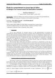
• The maximum range R max is defined as the depth at which extrapolation of the tail
of the central-axis depth dose curve meets the bremsstrahlung background, as
shown in Fig. 8.2. It is the largest penetration depth of electrons in the absorbing
medium. The maximum range has the drawback of not giving a well-defined
measurement point.
• The practical range R p is defined as the depth at which the tangent plotted through
the steepest section of the electron depth dose curve intersects with the
extrapolation line of the background due to bremsstrahlung, as shown in Fig. 8.2.
• The depths R 90 and R 50 are defined as depths on the electron percentage depth
dose curve at which the percentage depth doses beyond z max attain values of 90%
and 50%, respectively.
• The depth R q is defined as the depth where the tangent through the dose inflection
point intersects the maximum dose level as shown in Fig. 8.2.
• It is evident that the csda range is of marginal usefulness in characterizing the
depth of penetration of electrons into an absorbing medium. Scattering effects,
both between the incident electrons and nuclei of the absorbing medium as well as
between the incident electrons and orbital electrons of the absorbing medium,
cause electrons to follow very tortuous paths resulting in large variations in actual
penetration of electrons into the absorbing medium.
TABLE 8.I. Csda RANGES IN AIR AND WATER FOR VARIOUS
ELECTRON ENERGIES.
Electron energy
(MeV)
6
7
8
9
10
20
30
Csda range in air
(g/cm 2 )
3.255
3.756
4.246
4.724
5.192
9.447
13.150
Csda range in
water (g/cm 2 )
3.052
3.545
4.030
4.506
4.975
9.320
13.170
229

Chapter 8. Electron Beams: Physical and Clinical Aspects
FIG. 8.2. Typical electron beam percentage depth dose curve illustrating the definition of
R q , R p , R max , R 50 . and R 90 .
8.1.5. Build-up region (depths between surface and z max , i.e., 0 ≤ z ≤ z max )
The dose build-up in electron beams is much less pronounced than that of megavoltage
photon beams and results from the scattering interactions that the electrons experience with
atoms of the absorber. Upon entry into the medium (e.g., water), the electron paths are
approximately parallel. With depth their paths become more oblique with regard to the
original direction due to multiple scattering, resulting in an increase in electron fluence along
the beam central axis.
• In the collision process between electrons and atomic electrons, it is possible that
the kinetic energy acquired by the ejected electron is large enough (hard collision)
to cause further ionisation. In such a case, these electrons are referred to as
secondary electrons or delta (∆) rays and they also contribute to the build-up of
dose.
• As seen in Fig. 8.1, the surface dose of electron beams (in the range from 75 to
95%) is much higher than the surface dose for photon beams (< 30%), and the rate
at which the dose increases from the surface to z max is therefore less pronounced
for electron beams than for photon beams.
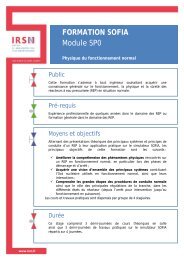
• Unlike in photon beams, the percent surface dose for electron beams increases
with electron energy. This can be explained by the nature of electron scatter. At
lower energies, the electrons are scattered more easily and through larger angles.
This causes the dose to build up more rapidly and over a shorter distance, as
shown in Fig. 8.3. The ratio of surface dose to maximum dose is, therefore, lower
for lower-energy electrons than for higher-energy electrons.
• In contrast to the behaviour of megavoltage photon beams, the depth of maximum
dose in electron beams, z max , does not follow a specific trend with electron beam
energy, rather it is a result of machine design and accessories used.
230

Review of Radiation Oncology Physics: A Handbook for Teachers and Students
FIG. 8.3. Percentage depth doses for electron beams of various energies (10 ×10 cm 2 field)
showing the increase in the surface dose with increasing energy.
8.1.6. Dose distribution beyond z max ( z > z max )
• Scattering and continuous energy loss by the electrons are the two processes
responsible for the sharp drop off in the electron dose at depths beyond z max .
• Bremsstrahlung produced in the head of the accelerator, in the air between the
accelerator window and the patient, and in the irradiated medium is responsible
for the "tail" in the depth dose curve.
• The range of electrons increases with increasing electron energy.
• The electron dose gradient is defined as follows: G = Rp /( Rp − Rq)
. The dose
gradient for lower electron energies is steeper than that for higher electron
energies, because the lower energy electrons are scattered at a greater angle away
from their initial directions.
• The bremsstrahlung contamination depends on electron beam energy, and is
typically less than 1% for 4 MeV and less than 4% for 20 MeV electron beams for
an accelerator with dual scattering foils.
8.2. DOSIMETRIC PARAMETERS OF ELECTRON BEAMS
8.2.1. Percentage depth dose
.
• Typical central axis PDD curves for various electron beam energies are shown in
Fig. 8.4 for a field size of 10 ×10 cm 2 .
• When diodes are used in PDD measurements, the diode signal represents the dose
directly because the stopping power ratio water-to-silicon is essentially
independent of electron energy.
231

Chapter 8. Electron Beams: Physical and Clinical Aspects
FIG. 8.4. Central axis PDD curves for a family of electron beams from a high energy linear
accelerator. All curves are normalized to 100% at z max .
• If an ionisation chamber is used in determination of electron beam depth dose
distributions, the measured depth ionisation distribution must be converted to a
depth dose distribution by using the appropriate stopping power ratios water-to-air
at depths in phantom.
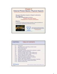
• When the distance between the central axis and the field edge is more than the
lateral range of scattered electrons, lateral scatter equilibrium exists and the depth
dose for a specific electron energy will be essentially independent of the field
dimensions, as shown in Fig. 8.5 for field sizes larger than 10×10 cm 2 and an
electron energy of 20 MeV.
• With decreasing field size an increasing degree of electronic disequilibrium will
be present at the central axis, and the depth dose and output factors will show
large sensitivity to field shape and size, as also shown in Fig. 8.5 for a 20 MeV
electron beam and field sizes smaller than 10×10 cm 2 .
• When the length of one side of the electron field decreases below the R p value for
a given electron energy, the depth of dose maximum decreases and the relative
surface dose increases with decreasing field size. The R p , on the other hand, is
independent of electron beam field size, as also shown in Fig. 8.5, and depends
only on electron beam energy.
232

Review of Radiation Oncology Physics: A Handbook for Teachers and Students
FIG. 8.5. PDD curves for different field sizes for a 20 MeV electron beam from a linear
accelerator. It is clearly illustrated that for field sizes larger than the practical range of the
electron beam (R p is about 10 cm for this 20 MeV electron beam), the PDD curve remains
essentially unchanged.
8.2.2. Oblique beam incidence
• The distributions in section 8.2.1 are given for normal beam incidence. For
oblique beam incidences with angles α between the beam central axis and the
normal to the phantom or patient surface exceeding 20 o , there are significant
changes to the PDD characteristics of the electron beam in contrast to the
behaviour observed in photon beams.
• Figure 8.6 illustrates the effect of the beam incidence angle α on PDD
distributions. Angle α = 0 represents normal incidence. The larger the angleα, the
shallower is z max and the larger is the dose at z max (beam output). All dose values
are normalized to 100% at z max for α = 0.
• For small angles of incidence α, the slope of the PDD curve decreases and the
practical range is essentially unchanged from that for normal beam incidence.
When the angle of incidence α exceeds 60 o , the shape of the PDD looses its
characteristic shape and the definition of R p can no longer be applied. For large
angles of incidence, the dose at z max increases significantly. This effect is due to
the increased electron fluence through the central axis from the oblique beam
angle.
233

Chapter 8. Electron Beams: Physical and Clinical Aspects
FIG. 8.6. PDD curves for various beam incidences for a 9 MeV (a) and 15 MeV (b) electron
beam. α = 0 represents normal beam incidence. The inset shows the geometry of the
experimental set-up and the doses at z max for various angles α relative to the dose at z max for
α = 0.
8.2.3. Output factors
• An important parameter that determines the electron beam output is the collimator
jaw setting. For each electron applicator (cone) there is an associated jaw setting
that is generally larger than the field size defined by the applicator (electron beam
cone). Such an arrangement minimizes the variation of collimator scatter and,
therefore, the output variation with field size is kept reasonably small. Typical
electron applicator sizes are 6×6; 10×10; 15×15; 20×20 and 25×25 cm 2 .
• The output factor for a given electron energy is the ratio of the dose for any
specific field size (applicator size) to the dose for a 10×10 cm 2 reference
applicator, both measured at z max .
• The square field defined by the applicator will not adequately shield all normal
tissues in most clinical situations. For this reason collimating blocks fabricated
from lead or a low melting point alloy are routinely inserted into the end of the
applicator to shape the fields. Output factors must also be measured for these
irregular fields.
• For small field sizes this extra shielding will affect the percentage depth dose and
the output factors due to lack of lateral scatter. The change in z max as well as
changes in the PDDs with small field sizes must be accounted for when measuring
output factors.
234

Review of Radiation Oncology Physics: A Handbook for Teachers and Students
8.2.4. Therapeutic range R 90
The depth of the 90% dose level (R 90 ) is defined as the therapeutic range for electron beam
therapy. The R 90 depth should, if possible, coincide with the distal treatment margin. This
depth is approximately given by E/4 in cm of water, where E is the nominal energy in MeV of
the electron beam. R 80 , the depth that corresponds to the 80% PDD, is also a frequently used
parameter for defining the therapeutic range, and can be approximated by E/3 in cm of water.
8.2.5. Electron beam energy specification
Because of the complexity of the spectrum, there is no single energy parameter that will fully
characterize the electron beam. Several parameters are used to describe the electron beam,
such as the most probable energy E p,o at the phantom or patient surface, the mean energy E
o
on the phantom or patient surface; and R 50 the depth at which the absorbed dose falls to 50%
of the maximum dose.
• The most probable energy E p,o on the phantom surface is empirically related to
the practical range R p in water as follows:
E p,o
= 0.22 +1.98 R p
+ 0.0025 R p
2
, (8.5)
where E p,o is in MeV and R p in cm.
• The mean electron energy Eo
depth R 50 as follows:
at the phantom surface is related to the half-value
E
= C R
0
, (8.6)
o 5
where C = 2.33 MeV/cm for water.
• The depth R 50 is calculated from the measured value of I 50 , the depth at which the
ionisation curve falls to 50% of its maximum, by
R 50 = 1.029 I 50 - 0.06 (cm) (for 2 ≤ I 50 ≤10 cm) (8.7)
R 50 = 1.059 I 50 - 0.37 (cm) (for I 50 >10 cm) (8.8)
• E
z
, the mean energy at a depth z in a water phantom is related to the practical
range R p by the Harder equation as follows:
Ez = Eo (1-z/ RP ) . (8.9)
8.2.6. Typical depth dose parameters as a function of energy
Some typical values for electron depth dose parameters as a function of energy are shown in
Table 8.II. These parameters should be measured for each electron beam before it is put into
clinical service.
235

Chapter 8. Electron Beams: Physical and Clinical Aspects
8.2.7. Profiles and off-axis ratios
A typical dose profile for a 6 MeV electron beam with a 25×25 cm 2 field at z max is shown in
Fig. 8.7. The off-axis ratio (OAR) relates the dose at any point in a plane, perpendicular to the
beam direction, to the dose on the central axis in that plane. A plot of OAR against the
distance from the central axis is referred to as a dose profile.
8.2.8. Flatness and symmetry
The specification for the flatness of electron beams according to the International Electrotechnical
Commission (IEC) is given at z max and consists of two requirements:
(1) The flatness specification requires that the distance between the 90% dose level
and the geometrical beam edge should not exceed 10 mm along the major axes
and 20 mm along the diagonals.
(2) The second requirement is that the maximum value of the absorbed dose
anywhere within the region bounded by the 90% isodose contour should not
exceed 1.05 times the absorbed dose on the axis of the beam at the same depth.
The specification for symmetry of electron beams according to IEC at z max is that the cross
beam profile should not differ by more than 2% for any pair of symmetric points with respect
to the central ray.
TABLE 8.II. TYPICAL DOSE PARAMETERS OF ELECTRON BEAMS.
Energy
(MeV)
R 90
(cm)
R 80
(cm)
R 50
(cm)
R p
(cm)
E 0
(MeV)
Surface dose
%
6 1.7 1.8 2.2 2.9 5.6 81
8 2.4 2.6 3.0 4.0 7.2 83
10 3.1 3.3 3.9 4.8 9.2 86
12 3.7 4.1 4.8 6.0 11.3 90
15 4.7 5.2 6.1 7.5 14.0 92
18 5.5 5.9 7.3 9.1 17.4 96
FIG. 8.7. Dose profile at depth z max for a 12 MeV electron beam and 25 × 25 cm 2 field.
236

Review of Radiation Oncology Physics: A Handbook for Teachers and Students
8.3. CLINICAL CONSIDERATIONS IN ELECTRON BEAM THERAPY
8.3.1. Dose specification and reporting
Electron beam therapy is usually applied to treatment of superficial or subcutaneous disease.
Treatments are usually delivered with a single direct electron field at a nominal source-skin
distance SSD of 100 cm.
• The dose specification for treatment is commonly given at a depth that lies at, or
beyond, the distal margin of the disease and the energy chosen for treatment
depends on the depth of the lesion to be treated.
• To maximise healthy tissue sparing beyond the tumour, while at the same time
providing relatively homogenous target coverage, treatments are usually
prescribed at either z max , R 90 , or R 80 .
• If the treatment dose is specified at either R 80 or R 90 , the skin dose will often be
higher than the prescription dose.
• The maximum dose to the patient could be up to 20% higher than the prescribed
dose. Therefore, the maximum dose should always be reported for electron beam
therapy.
8.3.2. Bolus – electron range modifier
Bolus is often used in electron beam therapy:
(a)
(b)
(c)
To increase the surface dose,
To flatten out irregular surfaces and
To reduce the electron beam penetration in some parts of the treatment field.
• For very superficial lesions, the practical range of even the lowest energy beam
available from a linac may be too large to provide adequate healthy tissue sparing
beyond the tumour depth. To overcome this problem, a tissue-equivalent bolus
material of specified thickness may be placed on the surface of the patient with
the intent to shorten the range of the beam in the patient.
• Bolus may also be used to define more precisely the range of the electron beam.
The difference between available electron beam energies from a linac is usually
no less than 3 or 4 MeV. If the lower energy is not penetrating enough, and the
next available energy is too penetrating, bolus may be used with the higher energy
beam to fine-tune the electron beam range.
8.3.3 Small field sizes
• For field sizes larger than the practical range of the electron beam, the PDD curve
remains constant with increasing field size, since the electrons from the periphery
of the field are not scattered sufficiently to contribute to the central axis depth
dose.
237

Chapter 8. Electron Beams: Physical and Clinical Aspects
• When the field is reduced below that required for lateral scatter equilibrium, the
dose rate decreases, z max moves closer to the surface and the PDD curve becomes
less steep (see Fig. 8.8). Therefore, for all treatments involving small electron
beam field sizes, the beam output as well as the full PDD distribution must be
determined for a given patient treatment.
8.3.4. Isodose curves
Isodose curves are lines passing through points of equal dose. Isodose curves are usually
drawn at regular intervals of absorbed dose and are expressed as a percentage of the dose at a
reference point that is normally taken as the z max point on the beam central axis. As an
electron beam penetrates a medium, the beam expands rapidly below the surface due to
scattering. However, the individual spread of the isodose curves varies depending on the
isodose level, energy of the beam, field size, and beam collimation.
• A particular characteristic of electron beam isodose curves is the bulging of the
low value curves (80%).
• Isodose curves for a 9 MeV and 20 MeV electron beam are shown in Fig. 8.9. The
phenomena of bulging and constricting isodose curves are clearly visible.
• The term penumbra generally defines the region at the edge of a radiation beam
over which the dose rate changes rapidly as a function of distance from the beam
central axis. The physical penumbra of an electron beam may be defined by the
distance between two specified isodose curves at a specified depth. A penumbra
defined in this way is a rapidly varying function of depth. The ICRU has
recommended that the 80% and 20% isodose lines be used in the determination of
the physical penumbra, and that the specified depth of measurement be R 85 /2
where R 85 is the depth of the 85% dose level on the electron beam central axis.
FIG. 8.8. Variation of the electron beam percentage depth dose with field size.
238

Review of Radiation Oncology Physics: A Handbook for Teachers and Students
FIG. 8.9. Measured isodose curves for 9 MeV and 20 MeV electron beams. The field size is
10×
10 cm
2 and SSD = 100 cm. Note the bulging low value isodose lines for both beam
energies. The 80% and 90% isodose lines for the 20 MeV beam exhibit a severe lateral
constriction.
• The low value isodose lines (for example, below the 50% isodose line) diverge
with increasing air gap between the patient and the end of the applicator (cone),
while the high value isodose lines converge toward the central axis. This means
that the penumbra will increase if the distance from the applicator increases.
8.3.5. Field shaping
Field shaping for electron beams is always achieved with electron applicators (cones) that
may be used alone or in conjunction with shielding blocks or special cutouts.
Electron applicators
• Normally the photon beam collimators on the accelerator are too far from the
patient to be effective for electron field shaping.
239

Chapter 8. Electron Beams: Physical and Clinical Aspects
• After passing through the scattering foil, the electrons scatter sufficiently with the
other components of the accelerator head, and in the air between exit window and
the patient to create a clinically unacceptable penumbra.
• Electron beam applicators or cones are usually used to collimate the beam, and are
attached to the treatment unit head such that the electron field is defined at
distances as small as 5 cm from the patient.
• Several cones are provided, usually in square field sizes ranging from 5×5 cm 2 to
25×25 cm 2 .
Shielding and cutouts
• For a more customised field shape, a lead or metal alloy cutout may be
constructed and placed on the applicator as close to the patient as possible.
• Standard cutout shapes may be pre-constructed and be ready for use at treatment
time.
• Custom cutout shapes may also be designed for patient treatment. Field shapes
may be determined from conventional or virtual simulation, but are most often
prescribed clinically by the physician prior to the first treatment.
• As a rule of thumb, simply divide the practical range R p by 10 to obtain the
approximate thickness of lead required for shielding (< 5% transmission).
• Lead thickness required for shielding of various electron energies with transmissions
of 50, 10, and 5% is given in Table 8.III.
Internal Shielding
• For certain treatments, such as treatment of the lip, buccal mucosa, eye lids or ear
lobes, it may be advantageous to use an internal shield to protect the normal
structures beyond the target volume.
• Care must be taken to consider the dosimetric effects of placing lead shielding
directly on patient’s surface. Electrons, back-scattered from the shielding, may
deliver an inadvertently high dose to healthy tissue in contact with the shield. This
dose enhancement can be appreciable and may reach levels of 30 to 70% but it
drops off exponentially with distance from the interface on the entrance side of the
beam.
• Aluminum or acrylic have been used around lead shields to absorb the backscattered
electrons. Often, these shields are dipped in wax to form a 1 mm or 2
mm coating around the lead. This not only protects the patient from the toxic
effects of lead, but also absorbs any scattered electrons which are usually low in
energy.
240

Review of Radiation Oncology Physics: A Handbook for Teachers and Students
TABLE 8.III. LEAD THICKNESS REQUIRED FOR VARIOUS TRANSMISSION
LEVELS (IN mm) FOR A 12.5×12.5 cm 2 FIELD.
Energy (MeV) 6 8 10 12 14 17 20
Transmission
50% 1.2 1.8 2.2 2.6 2.9 3.8 4.4
10% 2.1 2.8 3.5 4.1 5.0 7.0 9.0
5% 3.0 3.7 4.5 5.6 7.0 8.0 10.0
Extended SSD treatments
• In clinical situations where the set up at the nominal SSD is precluded, an
extended SSD might be used, although, as a general rule, one should avoid such
treatments unless absolutely necessary.
• Extending the SSD typically produces a large change in output, a minimal change
in PDD and a significant change in beam penumbra. The beam penumbra can be
restored by placing collimation on the skin surface. The inside edge of the skin
collimation has to be well within the penumbra cast by the normal treatment
collimator.
• Clinical electron beams are not produced at a single source position in the head of
the linac but rather as an interaction of a pencil beam with the scattering foil and
other components.
• In general, the inverse square law, as used for photon beams, cannot be applied to
electron beams without making a correction.
• A “virtual source” position for electron beams can be determined experimentally,
as the point in space that appears to be the point-source position for the electron
beam.
• An “effective” SSD, based on the “virtual source” position, is used when applying
the inverse square law to correct for a non-standard SSD.
8.3.6. Irregular surface correction
Isodose correction due to irregular patient shape
A frequently encountered situation in electron beam therapy is when the end of the treatment
cone is not parallel to the skin surface of the patient. This could result in an uneven air gap
and corrections would have to be made to the dose distribution to account for the sloping
surface. Corrections to isodose lines can be applied on a point by point basis through the use
of the following equation:
⎡ SSD + z ⎤
D SSDeff g,z Do SSD
eff
,z ⎢
⎥ OF ,z
⎣SSDeff
+ g + z ⎦
eff
( + ) = ( ) × ( θ )
2
, (8.10)
241

Chapter 8. Electron Beams: Physical and Clinical Aspects
where
SSD eff is the effective SSD,
g
is the air gap,
z
is the depth in the patient,
θ
is the the obliquity angle between the tangent to the skin surface and the beam
central axis,
D o
(SSD eff
, z) is the dose at depth z for a beam incident normally on a flat phantom and
OF(θ,z) is a correction factor for the obliquity of the beam that tends to unity for beams
of perpendicular incidence. This factor may either be measured or looked up in
the literature.
Bolus
A tissue-equivalent material, such as wax, can be used to physically remove irregularities in
the patient contour. The wax can be molded to the patient’s surface, filling-in the irregularities
and leaving a flat incidence for the electron beam.
Bolus can also be used to shape isodose lines to conform to tumour shapes.
• Sharp surface irregularities where the electron beam may be incident tangentially
give rise to a complex dose distribution with hot and cold spots. Tapered bolus
around the irregularity may be used to smooth out the surface and reduce the dose
inhomogeneity.
• Although labour-intensive, the use of bolus for electron beam treatments is very
practical, since treatment planning software for electron beams is limited, and
empirical data are normally collected only for standard beam geometries.
• The use of CT for treatment planning enables accurate determination of tumour
shape, depth, and patient contour. If a wax bolus can be constructed such that the
total distance from the surface of the bolus to the required treatment depth is
constant along the length of the tumour, then the shape of the resulting isodose
curves should approximate the shape of the tumour (see Fig. 8.10).
FIG. 8.10. Construction of a custom bolus to conform isodose lines to the shape of the target.
242

Review of Radiation Oncology Physics: A Handbook for Teachers and Students
8.3.7. Inhomogeneity corrections
The dose distribution from an electron beam can be greatly affected by the presence of tissue
inhomogeneities such as lung or bone. The dose within these inhomogeneities is difficult to
calculate or to measure, but the effect on the distribution beyond the inhomogeneity is
quantifiable.
Coefficient of equivalent thickness
• The simplest correction for tissue inhomogeneities involves the scaling of the
inhomogeneity thickness by its density relative to water, and the determination of
a coefficient of equivalent thickness (CET).
• The CET of a material is given by its electron density relative to the electron
density of water, and is essentially equivalent to mass density of the
inhomogeneity. For example, lung has an approximate density of 0.25 g/cm 3 and a
CET of 0.25. Thus, a thickness of 1 cm of lung is equivalent to 0.25 cm of tissue.
Solid bone has a CET of approximately 1.6.
• The CET can be used to determine an effective depth in water-equivalent tissue
z eff through the following expression:
z eff = z-t(1-CET) , (8.11)
where z is the actual depth of the point in the patient and t is the thickness of the
inhomogeneity.
• Figure 8.11 illustrates the effect of a lung inhomogeneity on the PDD curve of an
electron beam.
FIG. 8.11. Effect of a 5 cm lung inhomogeneity on a 15 MeV electron beam PDD.
243

Chapter 8. Electron Beams: Physical and Clinical Aspects
Scatter perturbation (edge) effects
• If an electron beam strikes the interface between two materials either tangentially
or at a large oblique angle, the resulting scatter perturbation will affect the dose
distribution at the interface. The lower density material will receive a higher dose
due to the increased scattering of electrons from the higher density side.
• Edge effects need to be considered in the following situations:
- Inside a patient, at the interfaces between internal structures of different
density.
- On the surface of the patient, in regions of sharp surface irregularity.
- On the interface between lead shielding and the surface of the patient, if the
shielding is placed superficially on the patient, or if it is internal shielding.
• The enhancement in dose at the tissue-metal interface is dependent on beam
energy at the interface and on the atomic number of the metal. In the case of
tissue-lead interface, the electron backscatter factor (EBF) is empirically given by:
EBF .
−0052
d
= 1+ 0 735e , E , (8.12)
where E d
is the average energy of electrons incident on the interface.
8.3.8. Electron beam combinations
Electron beams may be abutted to adjacent electron fields or to adjacent photon fields.
Abutted electron fields
• When abutting electron fields, it is important to take into consideration the
dosimetric characteristics of electron beams at depth. The large penumbra and
bulging isodose lines make hot spots and cold spots in the target volume
practically unavoidable.
• Contiguous electron beams should be parallel to each other to avoid significant
overlapping of the high value isodose curves at depth.
• In general, it is best to avoid adjacent electron fields, but if treatment of these
fields is absolutely necessary, some basic film dosimetry should be carried out at
the junction prior to treatment to verify that no hot or cold spots in dose are
present.
Abutted photon and electron fields
Electron-photon field matching is easier than electron-electron field matching. A distribution
for photon fields is usually available from a treatment planning system, and the location of the
electron beam treatment field as well as the associated hot spots and cold spots can be
determined relative to the photon field treatment plan. The matching of electron and photon
fields on the skin will produce a hot spot on the photon side of the treatment.
244

8.3.9. Electron arc therapy
Review of Radiation Oncology Physics: A Handbook for Teachers and Students
Electron arc therapy is a special radiotherapeutic technique in which a rotational electron
beam is used to treat superficial tumour volumes that follow curved surfaces. While the
technique is well known and accepted as clinically useful in the treatment of certain tumours,
it is not widely used because it is relatively complicated and its physical characteristics are
poorly understood. The dose distribution in the target volume depends in a complicated
fashion on electron beam energy, field width, depth of isocentre, source-axis distance, patient
curvature, tertiary collimation, and field shape as defined by the secondary collimator.
The excellent clinical results achieved by the few pioneers in this field during the past two
decades have certainly stimulated an increased interest in electron arc therapy, both for
curative treatments as well as for palliation. In fact, manufacturers of linacs now offer the
electron arc therapy mode as one of standard treatment options. While this option is usually
purchased with a new linac since it is relatively inexpensive, it is rarely used clinically
because of the technical difficulties involved.
• Two approaches to electron arc therapy have been developed: the simpler is
referred to as electron pseudo-arc and is based on a series of overlapping
stationary electron fields and the other uses a continuous rotating electron beam.
• The calculation of dose distributions in electron arc therapy is a complicated
procedure and usually cannot be performed reliably with algorithms used for
standard stationary electron beam treatment planning.
• The angle β concept offers a semiempirical technique to treatment planning for
electron arc therapy. The characteristic angle β for an arbitrary point A on the
patient's surface (Fig. 8.12) is measured between the central axes of two rotational
electron beams positioned in such a way that at point A the frontal edge of one
beam crosses the trailing edge of the other beam.
FIG. 8.12. Schematic representation of the arc therapy geometry: f is the source-axis
distance; d i the depth of isocentre; w, the field width defined at isocentre; α the arc angle or
the angle of treatment; and β the characteristic angle for the particular treatment geometry.
245

Chapter 8. Electron Beams: Physical and Clinical Aspects
• The angle β is uniquely determined by three treatment parameters: the sourceaxis
distance f, the depth of isocentre d i and the field width w. Electron beams with
combinations of d i and w which give the same characteristic angle β actually
exhibit very similar radial percentage depth doses even though they may differ
considerably in individual d i and w (see Fig. 8.13). Thus the percentage depth
doses for rotational electron beams depend only on the electron beam energy and
on the characteristic angleβ .
• Photon contamination is of concern in electron arc therapy, since the photon
contribution from all beams is added at isocentre and the isocentre might be
placed on a critical structure. Figure 8.14 shows a comparison between two dose
distributions measured with film in a humanoid phantom. Film (a) is for a small β
of 10 o , i.e., a small field width, and it clearly exhibits a large photon dose at
isocentre, while film (b) was taken for a large β of 100 o and exhibits a low photon
dose at isocentre. In arc therapy, the isocentre bremsstrahlung dose is inversely
proportional to the characteristic angle β.
FIG. 8.13. Radial percentage depth doses in electron arc therapy measured in phantom for
various combinations of w and d i giving characteristic angles β of (a) 20°, (b) 40°, (c) 80°
and (d) 100°. Electron beam energy: 9 MeV.
246

Review of Radiation Oncology Physics: A Handbook for Teachers and Students
FIG. 8.14. Dose distributions for a 15 MeV rotational electron beam with an isocentre depth
d i of 15 cm, (a) for a β of 10° and (b) for a β of 100°.
• One of the technical problems related to the electron arc treatment involves the
field shape of the moving electron beam defined by secondary collimators. For
the treatment of sites that can be approximated with cylindrical geometry (e.g.,
chest wall), the field width can be defined by the rectangular photon collimators.
However, when treating sites that can only be approximated with a spherical
geometry (e.g., scalp), a custom-built secondary collimator, defining a nonrectangular
field of appropriate shape has to be used to provide a homogeneous
dose in the target volume.
8.3.10. Electron therapy treatment planning
The complexity of electron-tissue interactions does not make electron beams well suited to
conventional treatment planning algorithms. Electron beams are difficult to model, and lookup
table type algorithms do not predict well the dose for oblique incidences or tissue
interfaces.
The early methods of electron dose distribution calculations were empirical and based on
water phantom measurements of percentage depth doses and beam profiles for various field
sizes, similarly to the Milan and Bentley method developed in the late 1960s for use in photon
beams. Inhomogeneities were accounted for by scaling the depth dose curves using the CET
technique. This technique provides useful parametrization of the electron depth dose curve but
has nothing to do with the physics of electron transport that is dominated by the theory of
multiple scattering.
The Fermi-Eyges multiple scattering theory considers a broad electron beam as being made
up of many individual pencil beams which spread out laterally in tissue, approximately as a
Gaussian function with the amount of spread increasing with depth. The dose at a particular
point in tissue is calculated by an addition of contributions of spreading pencil beams.
The pencil beam algorithm can account for tissue inhomogeneities, patient curvature and
irregular field shape. Rudimentary pencil beam algorithms dealt with lateral dispersion but
ignored angular dispersion and back-scattering from tissue interfaces. Subsequent analytical
advanced algorithms refined the multiple scattering theory through applying both the stopping
powers as well as the scattering powers but nevertheless generally failed to provide accurate
dose distributions in general clinical conditions.
247

Chapter 8. Electron Beams: Physical and Clinical Aspects
The most accurate way to calculate electron beam dose distributions is through Monte Carlo
techniques. The main drawback of the current Monte Carlo approach as a routine dose
calculation engine is its relatively long calculation time. However, with the ever-increasing
computer speed combined with the decreasing hardware cost, one can expect that in the near
future Monte Carlo based electron dose calculation algorithms will become available for
routine clinical applications.
BIBLIOGRAPHY
INTERNATIONAL COMMISSION ON RADIATION UNITS AND MEASUREMENTS,
(ICRU), “Radiation dosimetry: Electron beams with energies between 1 and 50 MeV”, ICRU
Report 35, ICRU, Bethesda, Maryland, U.S.A. (1984).
JOHNS, H.E., CUNNINGHAM, J.R., “The physics of radiology”, Thomas, Springfield,
Illinois, U.S.A. (1985).
KHAN, F.M., “The physics of radiation therapy”, Williams and Wilkins, Baltimore, Maryland,
U.S.A. (1994).
KLEVENHAGEN, S.C., “Physics and dosimetry of therapy electron beams”, Medical Physics
Publishing, Madison, Wisconsin, U.S.A. (1993).
248