Aerodynamic Coefficient Prediction of a General Transport Aircraft ...
Aerodynamic Coefficient Prediction of a General Transport Aircraft ...
Aerodynamic Coefficient Prediction of a General Transport Aircraft ...

You also want an ePaper? Increase the reach of your titles
YUMPU automatically turns print PDFs into web optimized ePapers that Google loves.
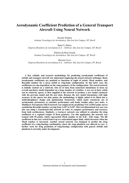
<strong>Aerodynamic</strong> <strong>Coefficient</strong> <strong>Prediction</strong> <strong>of</strong> a <strong>General</strong> <strong>Transport</strong><br />
<strong>Aircraft</strong> Using Neural Network<br />
Ricardo Wallach<br />
Instituto Tecnológico de Aeronáutica, São José dos Campos, SP, Brazil<br />
Bento S. Mattos<br />
Empresa Brasileira de Aeronáutica S.A. – Embraer, São José dos Campos, SP, Brazil<br />
Roberto da Mota Girardi<br />
Instituto Tecnológico de Aeronáutica, São José dos Campos, SP, Brazil<br />
Marcelo Curvo<br />
Empresa Brasileira de Aeronáutica S.A. – Embraer, São José dos Campos, SP, Brazil<br />
A fast, reliable, and accurate methodology for predicting aerodynamic coefficients <strong>of</strong><br />
airfoils and transport aircraft was elaborated employing the neural network technique. Basic<br />
aerodynamic coefficients are modeled as functions <strong>of</strong> angle <strong>of</strong> attack, Mach number, and<br />
Reynolds number for a given airfoil or wing-body configuration. In this latter case, the<br />
coefficients are also dependent on the wing geometry <strong>of</strong> the configuration. The neural network<br />
is initially trained on a relatively rich set <strong>of</strong> data from numerical simulations to learn an<br />
overall non-linear model dependent on a large number <strong>of</strong> variables. A new set <strong>of</strong> data, which<br />
can be relatively sparse, is then supplied to the network to produce a new model consistent<br />
with the previous model and the new data. Because the new model interpolates with high<br />
accuracy in the sparse test data points, the methodology is highly suited to be fitted into a<br />
multi-disciplinary design and optimization framework, which make extensively use <strong>of</strong><br />
aerodynamic parameters to calculate performance and loads, besides other core tasks. A<br />
Multilayer Perceptrons (MLP) network was employed for predicting NACA23012 polar curves<br />
considering Reynolds number varying from 1x10 6 to 5x10 6 . This two-dimensional test case was<br />
also run using a Functional-Link network in order to compare performance and accuracy<br />
from both architectures. Similarly, a two-layer network was utilized to calculate the drag<br />
coefficient <strong>of</strong> a regional twinjet <strong>of</strong> fixed geometry. For this application, the network was<br />
trained with 99 points, which represented Mach number in the 0.20 - 0.82 range. The lift<br />
coefficient in this case varied from 0 up to a determined upper limit, which decreases when the<br />
Mach number is increased. Another neural network was designed to predict the drag<br />
coefficient <strong>of</strong> a wing-fuselage combination, where the wing planform was allowed to vary. A<br />
further work for drag prediction <strong>of</strong> wing-fuselage configuration with generic airfoils and<br />
planform is currently under development.<br />
1<br />
American Institute <strong>of</strong> Aeronautics and Astronautics
Symbology and Abbreviations<br />
BL<br />
C d<br />
C D<br />
C l<br />
C L<br />
M<br />
Re<br />
α<br />
AR<br />
λ<br />
φ LE<br />
Y K<br />
CFD<br />
MDO<br />
FLN<br />
LMS<br />
LHS<br />
RBF<br />
MLP<br />
= Abbreviation for boundary layer<br />
= Two-dimensional drag coefficient<br />
= Three-dimensional drag coefficient<br />
= Two-dimensional lift coefficient<br />
= Three-dimensional lift coefficient<br />
= Mach number<br />
= Reynolds number<br />
= Angle <strong>of</strong> attack<br />
= Wing aspect ratio<br />
= Wing taper ratio<br />
= Wing leading-edge sweepback angle<br />
= Wing break position referred to wingspan<br />
= Computational fluid dynamics<br />
= Multi-disciplinary design and optimization<br />
= Functional link network<br />
= Least-mean square algorithm<br />
= Latin hypercube sampling<br />
= Radial basis function<br />
= Multi-layer perceptron<br />
I. Introduction<br />
The present work discusses the application <strong>of</strong> neural networks for accurately predicting aerodynamic coefficients<br />
<strong>of</strong> airfoil and wing-body configurations. Meta-models based on neural-network are able to handle non-linear<br />
problems with a large amount <strong>of</strong> variables. Some test cases were carried out in order to validate the entire procedure<br />
for aerodynamic coefficient prediction. The results indicate that it is possible to improve aircraft conceptual<br />
studies 6,7 , which make extensive use <strong>of</strong> aerodynamic calculations. The methodology is also suited for<br />
implementation into a multi-disciplinary aircraft design and optimization (MDO) framework. In this context, huge<br />
computer time savings without losing the required accuracy for the definition <strong>of</strong> the aircraft configuration were<br />
recorded.<br />
For centuries, the scientific approach for the understanding <strong>of</strong> physical laws was based on the construction <strong>of</strong><br />
mathematical models. Usually solving a non-linear system <strong>of</strong> equations, the behavior <strong>of</strong> physical phenomena could<br />
then be known. Mathematical models can be used to describe the behavior <strong>of</strong> the non-linear systems, considering<br />
initial conditions and boundary conditions are furnished. However, new simulation tools, among them neural<br />
networks, appeared and are providing new ways to predict system behavior. They represent a new computing<br />
paradigm based on the parallel architecture <strong>of</strong> the brain. Actually, neural network refers to a multifaceted<br />
representation <strong>of</strong> neural activity constituted by the essence <strong>of</strong> neurobiology, the framework <strong>of</strong> cognitive science, the<br />
art <strong>of</strong> computation, the physics <strong>of</strong> statistical mechanics, and the concepts <strong>of</strong> cybernetics. Inputs from these diverse<br />
disciplines have widened the scope <strong>of</strong> neural network modeling with the emergence <strong>of</strong> artificial neural networks and<br />
their engineering applications to pattern recognition and adaptive systems, which mimic the biological neural<br />
complex in being trained to learn from examples. Neural networks are universal function estimators that contain<br />
artificial neurons. The neurons are linked by adaptive interconnections, arranged in a large parallel architecture. This<br />
arrangement produces a weighted sum <strong>of</strong> the inputs and can be trained to produce an accurate output for a given<br />
input. This training consists <strong>of</strong> adjusting the weights applied by the network as it sums the inputs. The power <strong>of</strong><br />
neural networks lies in their ability to represent general relationships, and in their ability to learn these relationships<br />
directly from the data being modeled. There are essentially four broad categories <strong>of</strong> problems to which neural<br />
networks have applications: classification <strong>of</strong> patterns; function approximation; behavior prediction; and data mining.<br />
<strong>Aircraft</strong> design is a highly complex and time-consuming task involving several strongly coupled disciplines.<br />
Considering the current highly competitive aircraft market, it has become mandatory for new designs that they must<br />
be submitted to multi-disciplinary optimization process. Aeronautical industry design objectives usually are<br />
considered in the following order: obtaining a feasible and viable configuration; to perform a robust design task;<br />
achieving an improved configuration; an optimal aircraft. Due to all those reasons, genetic algorithms has become<br />
commonplace within MDO frameworks as well as acquired widespread use in many other applications. An usual<br />
2<br />
American Institute <strong>of</strong> Aeronautics and Astronautics
approach for MDO concerned with the use <strong>of</strong> genetic algorithms, which require a large amount – population – <strong>of</strong><br />
individuals, and the application <strong>of</strong> random mutations and crossing over <strong>of</strong> those individuals, for each generation <strong>of</strong><br />
this population 4 . This approach may lead to a huge amount <strong>of</strong> different designs, which should be individually<br />
evaluated in order to segregate Pareto-optimum solutions and discard unfeasible or non-efficient results. The<br />
performance <strong>of</strong> each aircraft is evaluated based on the calculation provided by different dedicated modules for every<br />
aspect being analyzed. The analysis modules adopted in airplane MDO problems usually comprise: aerodynamics;<br />
performance; stability and control; weight and structures and, ideally, acquisition and operating costs. <strong>Aerodynamic</strong><br />
characteristics <strong>of</strong> the population could be obtained by using analytical or semi-empirical methodologies provided by<br />
different authors 6,7 . This approach, however, presents a serious drawback: although usually qualitative results are<br />
correct, numerical results provided by such methods are highly unreliable, due to the inherent difficulty in modeling<br />
highly non-linear aerodynamic phenomena, as well as the frequent necessity <strong>of</strong> interpolating and even extrapolating<br />
relations provided by analysis <strong>of</strong> wind-tunnel experiments. Design based on these methods will never provide the<br />
level <strong>of</strong> accuracy required for MDO applied for aircraft design. In addition, in the usual approach, aerodynamics<br />
analysis <strong>of</strong> each individual in the population is done with complex and time-consuming CFD s<strong>of</strong>tware, which can be<br />
responsible for a large amount <strong>of</strong> the total time spent in the MDO process. For these reasons, a neural-network based<br />
meta-model seems to be more suited for aircraft conceptual studies. Implementing an aerodynamics module based<br />
on neural networks has further potential advantages over the usual CFD approach:<br />
1) The calculation <strong>of</strong> the aerodynamics coefficients by means <strong>of</strong> CFD analysis can be made only for the<br />
training set <strong>of</strong> individuals, thus dramatically reducing the amount <strong>of</strong> computational effort required for the<br />
overall design process. In this case, the coefficient values for the rest <strong>of</strong> the population are obtained much<br />
faster, by interpolating the results <strong>of</strong> the training set by means <strong>of</strong> a properly trained and validated neural<br />
network;<br />
2) The reduction in computation time provided by a neural net aerodynamic data bank could also allow<br />
increasing the size <strong>of</strong> the population under consideration and the number <strong>of</strong> generations, thus leading a<br />
broader range <strong>of</strong> available quasi-optimum solutions for the proposed problem;<br />
3) No necessity to retrain the network from scratch every time a new project begins. Neural networks can be<br />
trained accumulatively, by using the so-called adaptative learning algorithms. Thus, knowledge<br />
accumulated in past can always be recycled and expanded. This principle is granted by the minimum<br />
disturbance principle implemented in the LMS algorithm 5 ;<br />
4) For the cumulative training <strong>of</strong> the network, data from multiple sources, such as CFD analysis, wind tunnel<br />
and flight tests can be simultaneously used as input. In this case, special attention must be taken in order<br />
to hierarchically classify data based on its origin and reliability.<br />
The most usual networks employed for function approximation are the multi-layer perceptrons (MLP), the<br />
functional-link Networks (FLN), and the radial basis functions networks (RBF). All these architectures are very<br />
efficient in performing data regression, and can be trained in order to output data with a desired precision 1 .<br />
Multi-layer perceptrons are formed <strong>of</strong> at least two layers <strong>of</strong> neurons. In order to the network to be able <strong>of</strong><br />
approximating non-linear functions, it is important to have at least one hidden layer <strong>of</strong> neurons with non-linear<br />
transfer functions. The output layer <strong>of</strong> the MLP network is usually composed <strong>of</strong> neurons with linear transfer<br />
functions, in order to allow a broad range <strong>of</strong> output values. MLPs, as well as other classes <strong>of</strong> neural networks, can be<br />
fully or partially connected, and can be optimized in order to eliminate useless links, thus reducing the number <strong>of</strong><br />
parameters in the net and allowing faster calculations.<br />
In the functional link network, the hidden layer performs a functional expansion on the inputs, which gives the<br />
possibility to attach a physical meaning to the network parameters 3 . The approximation capability <strong>of</strong> an FLN<br />
depends on the chosen set <strong>of</strong> model basis that forms the hidden layer. Provided that the set <strong>of</strong> model bases is<br />
sufficiently rich (contains sufficient higher-order terms), it can be said that any continuous function can be<br />
uniformly approximated to certain accuracy. The FLNs are also linear in the parameters, which means that these<br />
parameters can always be learned in the least-square sense 2 .<br />
Radial basis function neural networks are other major class <strong>of</strong> neural network model - in which the distance<br />
between the input vector and a prototype vector determines the activation <strong>of</strong> a hidden unit. RBF networks are<br />
excellent regressors, and are usually single-layered structures, which can be trained faster to the desired accuracy.<br />
3<br />
American Institute <strong>of</strong> Aeronautics and Astronautics
II. Network Architecture<br />
For the test cases that studied, multi-layer non-linear perceptrons networks were employed. The networks were<br />
developed using Matlab ® , which contains a large number <strong>of</strong> sophisticated algorithms for training and optimization<br />
<strong>of</strong> this type <strong>of</strong> network, allowing greater flexibility in design and performance, as well as ease <strong>of</strong> implementation,<br />
compared to FLNs and RBFs set up in the same language.<br />
As stated before, the networks studied in this paper were set up as MLPs. However, the architectures<br />
implemented for both cases are different in terms <strong>of</strong> layers arrangement, number <strong>of</strong> neurons and transfer functions.<br />
It is not possible to set up deterministically the architecture <strong>of</strong> a non-linear network. In this case, the output layer<br />
is defined by the outputs <strong>of</strong> the problem being studied. The characteristics <strong>of</strong> the hidden layers must be defined as a<br />
compromise between the network size, the accuracy, and precision <strong>of</strong> the generated output and the training time, as<br />
well as overtraining and oscillatory behavior avoidance.<br />
A trial and error procedure was employed for the test cases under consideration for the definition <strong>of</strong> the network<br />
architecture. The procedure algorithm compares different possibilities and chooses that with best balance between<br />
the resulting performance goal (mean square error <strong>of</strong> the outputs) and normality <strong>of</strong> distribution <strong>of</strong> the resulting<br />
errors.<br />
A. NACA23012 Airfoil<br />
Inputs: Re; α; outputs: C l ; C d<br />
In a first approach, a two-layered network was employed. However, this layout was unable to resolve the acute<br />
bend present in the drag polar <strong>of</strong> the airfoil due to the free transition <strong>of</strong> the boundary layer at angle <strong>of</strong> attack close to<br />
zero lift. For this reason, a more complex design methodology was adopted. In order to approximate the existing<br />
relationship between the provided inputs and outputs, a three-layered network was adopted with the following<br />
layout:<br />
B. <strong>Transport</strong> Twinjet<br />
Layer 1 2 3<br />
Number <strong>of</strong> neurons 5 5 2<br />
Transfer function Tangent-sigmoid Log-sigmoid Pure linear<br />
Table 1. Network structure for the NACA 23012 Airfoil.<br />
Inputs: Re, M, and C L ; output: C D<br />
The drag polar <strong>of</strong> an airplane is normally a smooth, well-behaved curve. For that reason, a simple two-layered<br />
network was able to produce excellent interpolation results in this case, and the following layout was adopted:<br />
C. Wing-body configuration with generic wing geometry<br />
For this case, inputs can be divided in two groups:<br />
• Wing geometry: AR, λ, φ LE ,, and Y K .<br />
• Flow condition: M, Re, and C L .<br />
The output is the drag coefficient C D .<br />
Layer 1 2<br />
Number <strong>of</strong> neurons 10 1<br />
Transfer function Log-sigmoid Pure linear<br />
Table 2. Network structure for the NACA 23012 Airfoil.<br />
After many different attempts, the network architecture was defined according to the following table, and<br />
presented a good compromise between accuracy <strong>of</strong> the modeled phenomenon for the training set and small<br />
oscillatory behavior for the validation data set (without overtraining).<br />
4<br />
American Institute <strong>of</strong> Aeronautics and Astronautics
III. Training<br />
Training <strong>of</strong> a neural network is the process <strong>of</strong> adjusting the network’s gains and biases in order to obtain outputs<br />
as close as possible to the known target results for the training set <strong>of</strong> inputs. This array <strong>of</strong> inputs and corresponding<br />
expected outputs in known as the training set. The quality <strong>of</strong> the resulting outputs is evaluated by measuring the<br />
squared mean error <strong>of</strong> the network results compared to the targets, and the training algorithm is an optimization<br />
process, which tries to minimize this objective function, thus, the training procedure is also known as Least mean<br />
square. Moreover, the resulting errors are used as correction factors for the recalculation <strong>of</strong> the weights <strong>of</strong> the<br />
internal connections <strong>of</strong> the network, and those errors are propagated through the network from the output to the<br />
input layer, in a process so called back propagation.<br />
Neural networks can be trained simultaneously with a large training set (batch training), or accumulatively, by<br />
improving the network adding one point each time (adaptative training). In the cases when the training set is known<br />
before start <strong>of</strong> the process, batch training is preferable, due to its computational efficiency compared to adaptative<br />
methods. The optimization process <strong>of</strong> the LMS algorithm can be solved by several methods. For this paper, the<br />
chosen methodology was the Levenberg-Marquardt algorithm, which is an implementation <strong>of</strong> a quasi-Newton<br />
method, with variable learning rate. This algorithm ensures convergence, as in the steepest descent method, and has<br />
good performance, as does the Gauss-Newton algorithm.<br />
A. NACA 23012 Airfoil<br />
The training set <strong>of</strong> inputs and outputs for the airfoil was generated using the s<strong>of</strong>tware XFOIL 9 with the free<br />
laminar-turbulent boundary layer transition. The array consists <strong>of</strong> 125 points, generated according to the following<br />
schedule:<br />
B. <strong>Transport</strong> Twinjet<br />
Layer 1 2 3<br />
Number <strong>of</strong> neurons 20 10 1<br />
Transfer function Tangent-sigmoid Tangent-sigmoid Pure linear<br />
Table 3. Network structure for the Wing-fuselage configuration.<br />
Parameter Minimum value Maximum Value<br />
Re 1,000,000 6,000,000<br />
a -3 o 18 o<br />
Table 4. Training set – NACA 23012 Airfoil<br />
Training data for the network that models the drag polar <strong>of</strong> the regional jet was obtained by applying Class-II<br />
drag breakdown methodology, which consists in calculating drag coefficients for each isolated component <strong>of</strong> the<br />
airplane (e. g., wing, fuselage, etc.) and combining those components, plus interference and dynamic pressure<br />
correction factors, to obtain the total drag coefficient <strong>of</strong> the aircraft. This training set consists <strong>of</strong> 99 points <strong>of</strong> inputs<br />
and its corresponding expected outputs, arranged according to the following schedule:<br />
M 0.2 0.3 0.4 0.5 0.6 0.7 0.78 0.82<br />
Min Re 1.21E+07 1.26E+07 1.68E+07 1.48E+07 1.27E+07 1.12E+07 1.25E+07 1.32E+07<br />
Max Re 1.25E+07 1.88E+07 2.50E+07 3.13E+07 3.76E+07 4.39E+07 4.89E+07 5.14E+07<br />
Min C L 0 0 0 0 0 0 0 0<br />
Max C L 1.50 1.10 0.70 0.70 0.70 0.65 0.55 0.50<br />
Table 5. Training set – Regional jet<br />
5<br />
American Institute <strong>of</strong> Aeronautics and Astronautics
C. Wing-body configuration with variable wing geometry<br />
Data for training the network that models the drag coefficient <strong>of</strong> a wing-body configuration was generated using<br />
the structured full-potential code FPWB, which employs an approximate factorization algorithm for the time<br />
marching. A total <strong>of</strong> 1300 different wing geometries and flow conditions were simulated, covering a broad range <strong>of</strong><br />
inputs, with special attention to transonic flow conditions. This data set was generated according to a DOE technique<br />
named Latin Hypercube Sampling, or simply LHS algorithm 8 , which tries to ensure proper spatial distribution <strong>of</strong> the<br />
data, thus maximizing coverage <strong>of</strong> the parameters’ envelope (Table 6) with minimum correlation between samples<br />
AR l f LE Y K M Re C L<br />
Min. Value 5 0.15 0º 0.25 0.20 5E+06 0.30<br />
Max. Value 12 0.75 45º 0.60 0.82 4E+07 0.70<br />
Table 6. Training set – Wing/Fuselage configuration<br />
IV. Validation<br />
In order to validate the modeling capacities <strong>of</strong> the networks, auxiliary sets <strong>of</strong> points were generated.<br />
A. NACA 23012 Airfoil<br />
The validation data for this problem consists <strong>of</strong> 500 cases (125 from training + 375 additional points), which<br />
were generated by XFOIL, using the same schedule from section III.A. From the analysis <strong>of</strong> this data set, results the<br />
following statistical data. Table 7 shows the resulting error (known target minus network answer) associated with<br />
each output. As can be seen, the results for both output parameters show very small errors, with average close to<br />
zero and very small standard deviation.<br />
1. Drag <strong>Coefficient</strong><br />
Figure 1 shows a linear fit between expected target outputs and the results provided by the neural network. This<br />
figure shows that there is an excellent correspondence between expected and resulting outputs for the neural<br />
network.<br />
Associated Parameter C d<br />
Average 0.00005<br />
Standard Deviation 0.00016<br />
Maximum 0.0016<br />
Table 7. Validation Results – C d<br />
Figure 2 is the histogram <strong>of</strong> the errors. It shows that, as<br />
expected from the result in Table 5, the average <strong>of</strong> the<br />
errors is very close to zero, and have small standard<br />
deviation. Figure 3 shows the normal probability<br />
distribution <strong>of</strong> the errors for the outputs compared to the<br />
expected values. As can be seen, the resulting errors for the<br />
drag coefficient <strong>of</strong> the airfoil show an almost normal<br />
distribution. Moreover, the network does not show signal<br />
<strong>of</strong> excess <strong>of</strong> parameters or oscillatory behavior <strong>of</strong> results.<br />
Figure 1. Validation fit – C d . Comparison<br />
between expected outputs and network<br />
outputs for drag coefficient.<br />
6<br />
American Institute <strong>of</strong> Aeronautics and Astronautics
Figure 2. Histogram <strong>of</strong> residuals – C d . Histogram <strong>of</strong><br />
residuals for the drag coefficient <strong>of</strong> NACA23012<br />
airfoil.<br />
Figure 3. NPP <strong>of</strong> residuals – C d . Normal probability<br />
plot <strong>of</strong> residuals for the drag coefficient <strong>of</strong><br />
NACA23012 airfoil.<br />
2. Lift <strong>Coefficient</strong><br />
For the lift coefficient, a similar statistical analysis is presented:<br />
Associated Parameter C l<br />
Average 0.0002<br />
Standard Deviation 0.0052<br />
Maximum 0.029<br />
Table 8. Validation Results – C l<br />
For the lift coefficient, the histogram <strong>of</strong> the errors<br />
(Figure 5) shows heavy concentration <strong>of</strong> points around the<br />
average, which is also very close to zero. However, the<br />
normal probability plot <strong>of</strong> residuals (Figure 6) indicates that<br />
these errors do not appear to follow a Gaussian distribution.<br />
In this case, it is important to notice that statistical<br />
assumptions based on normal probability distributions cannot<br />
be stated. This fact does not invalidate the results, as can be<br />
seen in Figure 4, since there is still an excellent correlation<br />
between expected results and the neural network’s answers<br />
for the corresponding inputs. As in the case <strong>of</strong> the drag<br />
coefficient, there is no indication <strong>of</strong> oscillatory behavior <strong>of</strong><br />
the results.<br />
Figure 4. Validation fit – C d . Comparison<br />
between expected outputs and prediction<br />
by the network.<br />
7<br />
American Institute <strong>of</strong> Aeronautics and Astronautics
Figure 5. Histogram <strong>of</strong> residuals – C l . Histogram<br />
<strong>of</strong> residuals for the lift coefficient <strong>of</strong> NACA23012<br />
airfoil.<br />
Figure 6. NPP <strong>of</strong> residuals – C l . Normal<br />
probability plot <strong>of</strong> residuals for the lift coefficient <strong>of</strong><br />
NACA23012 airfoil.<br />
B. <strong>Transport</strong> Twinjet<br />
Validation data for the aircraft was also generated using a class-II drag polar generation approach. It consists <strong>of</strong><br />
396 points (99 from learning + 297). Table 9 shows statistical data associated with the error relating the expected<br />
outputs <strong>of</strong> the net to the corresponding answers. In this case, the only output provided by the network is the drag<br />
coefficient <strong>of</strong> the complete aircraft. Figure 7 shows excellent fit relating the expected outputs and the answers<br />
produced by the network.<br />
Associated Parameter C D<br />
Average -0.0000007<br />
Standard Deviation 0.00006<br />
Maximum 0.0007<br />
Table 9. Validation Results – C D<br />
Figure 8 shows the histogram <strong>of</strong> errors for the results<br />
produced by this network compared to the expected outputs.<br />
As in the case <strong>of</strong> the airfoil, the average <strong>of</strong> errors is very<br />
close to zero and the standard deviation <strong>of</strong> these errors is<br />
very small, actually less than 1 drag count. In addition,<br />
Figure 9 shows that these errors closely follow a Gaussian<br />
distribution, so it is proper to say that more than 99% <strong>of</strong> the<br />
results outputed by the network for the validation data set<br />
have associated errors smaller than 2 drag counts (three<br />
standard deviations).<br />
Figure 7. Validation fit – C D . Comparison<br />
between expected outputs and the predicted<br />
values from the neural network.<br />
8<br />
American Institute <strong>of</strong> Aeronautics and Astronautics
Figure 8. Histogram <strong>of</strong> residuals – C d . Histogram <strong>of</strong><br />
residuals for the drag coefficient <strong>of</strong> NACA23012<br />
airfoil.<br />
Figure 9. NPP <strong>of</strong> residuals – C D . Normal probability<br />
plot <strong>of</strong> residuals for the drag coefficient <strong>of</strong><br />
NACA23012 airfoil.<br />
B. Wing-body configuration with variable wing geometry<br />
Information used in the validation <strong>of</strong> the network that models the drag coefficient <strong>of</strong> the wing-body<br />
configuration was generated using the same method <strong>of</strong> the training set. This data set consists <strong>of</strong> 1550 cases, covering<br />
the same parameters schedule <strong>of</strong> the training set (Table 6).<br />
Statistical data associated to the residuals resulting <strong>of</strong> comparison between the C D generated by CFD analysis<br />
with FPWB code and its corresponding values as modeled by the proposed neural network can be found in Table<br />
10. It shows that the mean <strong>of</strong> the residuals is close to zero, and that the maximum error found for the validation data<br />
set was <strong>of</strong> nearly 18 drag counts.<br />
Associated Parameter C D<br />
Average<br />
4.02e-06<br />
Standard Deviation 0.00016<br />
Maximum 0.00177<br />
Table 10. Validation Results – C D .<br />
Figure 10 shows the histogram plot <strong>of</strong> the errors associated with the C D <strong>of</strong> the wing-body configuration with<br />
generic wing geometry, loading and flow condition. Figure 11 shows the fit between the target values <strong>of</strong> the drag<br />
coefficient (validation set only – generated with CFD) and the corresponding outputs <strong>of</strong> the neural network. As can<br />
be seen in this graph, there is an excellent correlation. Figure 12 is the normal probability plot <strong>of</strong> the residuals. It<br />
shows that the resulting distribution <strong>of</strong> errors cannot be considered normal. However, due to the good results <strong>of</strong> the<br />
fitting in Figure 11 and the overall low value <strong>of</strong> errors shown in Figure 13, which indicates that more than 97% <strong>of</strong><br />
the points have associated errors smaller than 5 drag counts, the resulting meta-model can be considered to be very<br />
good, specially for aircraft conceptual studies.<br />
9<br />
American Institute <strong>of</strong> Aeronautics and Astronautics
Figure 10. Histogram <strong>of</strong> residuals – C d . Histogram<br />
<strong>of</strong> residuals for the drag coefficient <strong>of</strong> the wing-body<br />
configuration.<br />
Figure 11. Validation fit – C D . Comparison<br />
between expected outputs and network answers<br />
for the drag coefficient <strong>of</strong> the wing-body<br />
configuration.<br />
Figure 12. NPP <strong>of</strong> residuals – C D . Normal probability<br />
plot <strong>of</strong> residuals for the drag coefficient <strong>of</strong> the wingbody<br />
configuration.<br />
Figure 13. Cumulative probability <strong>of</strong> errors – C D .<br />
Percentage <strong>of</strong> points with error smaller or equal than<br />
a give value, in drag counts, for the wing-body<br />
configuration.<br />
V. Simulation Examples<br />
In order to verify the modeling capacities <strong>of</strong> the networks, some drag polars and drag coefficient curves were<br />
generated, with input data that was not used for the learning processes. For the NACA 23012 airfoil, C l vs α curves<br />
were also generated, and compared to the corresponding data produced by the XFOIL code. For the wing-body<br />
configuration, testing points were also generating with FPWB28.<br />
A. NACA 23012 Airfoil<br />
Curves for this airfoil were generated for Reynolds numbers <strong>of</strong> 1.5 x 10 6 , 2.5 x 10 6 , and 4.5 x 10 6 . Alternatively,<br />
for Re=2.5 x 10 6 , the results are compared to that obtained by a properly trained functional-link network stated in<br />
terms <strong>of</strong> 34 functions connected by 7 th order polynomials. In Figures 16 and 17, it is possible to confront the results<br />
<strong>of</strong> the MLP and FL networks, and also a direct comparison between them and the simulation outputs produced by<br />
XFOIL.<br />
10<br />
American Institute <strong>of</strong> Aeronautics and Astronautics
From Figure 16, it is possible to see that both neural networks can resolve the lift curve <strong>of</strong> the airfoil with<br />
excellent accuracy, even for the prediction <strong>of</strong> the maximum C l , a highly non-linear characteristic <strong>of</strong> the wing section.<br />
In Figure 17, however, it is clear that the MLP net has better capacity <strong>of</strong> resolving the free BL transition fracture in<br />
the drag polar when compared to the FLN.<br />
1. Re=1.5x10 6 ; M=0.20<br />
Figure 14. C l vs a - NACA 23012. Lift coefficient<br />
versus angle <strong>of</strong> attack <strong>of</strong> the airfoil. Plotted for<br />
Re=1.5 x 10 6 and Mach number <strong>of</strong> 0.20.<br />
Figure 15. Drag polar – NACA 23012. Drag versus<br />
Lift coefficient curve <strong>of</strong> the airfoil. Plotted for Re=1.5<br />
x 10 6 and M=0.20 with free BL transition.<br />
2. Re=2.5 x 10 6 ; M=0.20<br />
Figure 16. C l vs a - NACA 23012. Lift coefficient<br />
versus angle <strong>of</strong> attack <strong>of</strong> the airfoil. Plotted for<br />
Re=2.5x10 6 and M=0.20. Comparison between FLN<br />
and MLP networks.<br />
Figure 17. Drag polar – NACA 23012. Drag versus<br />
Lift coefficient curve <strong>of</strong> the airfoil. Plotted for Re=2.5<br />
x 10 6 and M=0.20 with free BL transition.<br />
Comparison between FLN and MLP networks.<br />
11<br />
American Institute <strong>of</strong> Aeronautics and Astronautics
3. Re=4.5 x10 6 ; M=0.20<br />
Figure 18. C l vs a - NACA 23012. Lift coefficient<br />
versus angle <strong>of</strong> attack. Re=4.5 x 10 6 and M=0.20.<br />
Figure 19. Drag polar – NACA 23012. Drag versus<br />
Lift coefficient curve <strong>of</strong> the airfoil. Plotted for Re=4.5<br />
x 10 6 and M=0.20 with free BL transition.<br />
B. Twinjet Airliner<br />
In order to demonstrate the interpolation capabilities <strong>of</strong> the neural network drag polars <strong>of</strong> a twinjet airliner were<br />
estimated. The polars presented in this section were obtained with combinations <strong>of</strong> Reynolds and Mach number<br />
values that were not used in the network training process. A comparison to a Class-II methodology estimation for<br />
the same input can be seen in Fig. 20, The largest difference to the Class-II methodology was <strong>of</strong> 3 drag counts<br />
(Figure 22, @ C L =0).<br />
1. M=0.35; Re=1.75 x 10 7<br />
Figure 20. Drag polar <strong>of</strong> a Regional Jet. Lift versus drag coefficients<br />
for the twinjet airliner. M=0.35, Re=1.75 x 10 7 .<br />
12<br />
American Institute <strong>of</strong> Aeronautics and Astronautics
2. M=0.55; Re=2.00 x 10 7<br />
Figure 21. Drag polar <strong>of</strong> a Regional Jet. Lift versus drag coefficients<br />
for a new generation regional jet. Curve plotted for M=0.55 and<br />
Re=2.00 x 10 7 .<br />
3. M=0.75; Re=2.50x10 7 Figure 22. Drag polar <strong>of</strong> a <strong>Transport</strong> Twinjet. Lift versus drag<br />
coefficients for a new generation regional jet. Curve plotted for M=0.75<br />
and Re=2.5 x 10 7 .<br />
13<br />
American Institute <strong>of</strong> Aeronautics and Astronautics
C. Wing-body configuration with generic wing geometry<br />
The following figures show results for the simulation <strong>of</strong> the effect <strong>of</strong> changing the geometry <strong>of</strong> the wing and the<br />
flow over it, with a constant geometry fuselage. In each figure, the parameter indicated in the x-axis changes, and all<br />
the other remained six input variables are kept constant, with their corresponding values indicated in the title <strong>of</strong> the<br />
chart.<br />
Figures 23 to 29 show the effect <strong>of</strong> varying the wing geometry and flow condition for a typical transonic twinjet<br />
configuration. Figures 30 to 36 show these effects on typical regional turboprop airplane geometries. Figure 37<br />
shows the parameters adopted in the description <strong>of</strong> the wing geometry.<br />
FP<br />
Figure 23. C D vs AR – Wing-body configuration.<br />
Drag coefficient versus wing aspect ratio.<br />
Figure 24. C D vs l – Wing-body configuration.<br />
Drag coefficient versus wing taper ratio.<br />
Figure 25. C D vs f LE – Wing-body configuration.<br />
Drag coefficient versus wing leading edge sweep<br />
angle.<br />
Figure 26. C D vs Y K – Wing-body configuration.<br />
Drag coefficient versus the location <strong>of</strong> the wing<br />
break station.<br />
14<br />
American Institute <strong>of</strong> Aeronautics and Astronautics
Figure 27. C D vs C L – Wing-body configuration.<br />
Drag polar.<br />
Figure 28. C D vs Re – Wing-body configuration.<br />
Drag coefficient versus flight Reynolds’ number.<br />
Figure 29. C D vs Mach – Wing-body configuration.<br />
Transonic drag.<br />
Figure 30. C D vs AR – Wing-body configuration.<br />
Drag coefficient versus wing aspect.<br />
15<br />
American Institute <strong>of</strong> Aeronautics and Astronautics
Figure 31. C D vs l – Wing-body configuration.<br />
Drag coefficient versus wing taper.<br />
Figure 32. C D vs f LE – Wing-body configuration.<br />
Drag coefficient versus wing leading edge sweep<br />
angle.<br />
Figure 33. C D vs Y K – Wing-body configuration.<br />
Drag coefficient versus wing break position.<br />
Figure 34. C D vs Mach – Wing-body configuration.<br />
Transonic drag rise.<br />
16<br />
American Institute <strong>of</strong> Aeronautics and Astronautics
Figure 35. C D vs Re – Wing-body configuration.<br />
Drag coefficient versus flight Reynolds number.<br />
Figure 36. C D vs Mach – Wing-body configuration.<br />
Transonic drag rise.<br />
Figure 37. Top right, the chosen parameters for the definition <strong>of</strong> the wing<br />
geometry. Solid lines: real wing. Dashed lines: reference wing (used for calculation<br />
<strong>of</strong> the taper ratio as input variable only).<br />
17<br />
American Institute <strong>of</strong> Aeronautics and Astronautics
VI. Concluding Remarks<br />
From the results presented in the previous sections, it is possible to conclude that the implemented networks<br />
have excellent capacities for modeling the studied aerodynamic characteristics <strong>of</strong> the NACA 23012 airfoil, the<br />
complete airplane with fixed geometry and the wing-body configuration with generic wing geometry. The<br />
simulations showed that the relatively simple network structures implemented were able to resolve the highly nonlinear<br />
behavior <strong>of</strong> the phenomena under consideration, even for the high degree <strong>of</strong> precision required for<br />
applications in multi-disciplinary optimization design problems. This reveals that are room for a growth in the<br />
number <strong>of</strong> variable, necessary to handle realistic aircraft configurations.<br />
The comparison <strong>of</strong> the drag polars <strong>of</strong> the NACA 23012 airfoil generated with the 7 th order polynomial FLN and<br />
the MLP networks showed that the later are better suited for the solution <strong>of</strong> problems with pronounced non-linear<br />
characteristics. Thus, the results presented in this paper indicate that the MLP network architecture is probably<br />
adequate for the work <strong>of</strong> predicting the drag coefficient <strong>of</strong> an aircraft based on its geometry and flight condition,<br />
conclusion that is supported by the excellent results obtained for the wing-body configuration where the wing<br />
geometry was allowed o vary.<br />
References<br />
1. Arbib, M.A., The Handbook <strong>of</strong> Brain Theory and Neural Networks. Second Edition ed. 2003, Cambridge<br />
Massachussets: The MIT Press. 1301.<br />
2. Curvo, M. and Rios Neto, A. <strong>Aerodynamic</strong> Modeling and Stochastic Adaptative Control <strong>of</strong> High<br />
Performance <strong>Aircraft</strong> Using Artificial Neural Network and Parameter Identification. 2001, INPE - Instituto<br />
Nacional de Pesquisas Espaciais: São José dos Campos - Brazil.<br />
3. Curvo, M. and Rios Neto, A. Use <strong>of</strong> Functional Link Network in <strong>Aerodynamic</strong> Modeling <strong>of</strong> <strong>Aircraft</strong>. in 16th<br />
Brazilian Congress <strong>of</strong> Mechanical Engineering. 2001.<br />
4. Isikveren, A.T., Quasi-Analytical Modelling and Optimisation Techniques for <strong>Transport</strong> <strong>Aircraft</strong> Design, in<br />
Department <strong>of</strong> Aeronautics. 2002, Royal Institute <strong>of</strong> Technology (KTH): Stockholm, Sweden. p. 354.<br />
5. Kröse, B. and P.v.d. Smagt, An Introduction to Neural Networks. Eighth Edition ed. 1996, Amsterdam -<br />
Netherlands: The University <strong>of</strong> Amsterdam.<br />
6. Roskam, J., Airplane Design - Part VI. Airplane Design. Vol. 6. 1985, Ottawa, Kansas: DAR Corporation.<br />
7. Torenbeek, E., Synthesis <strong>of</strong> Subsonic Airplane Design. 1982, Rotherdam, Netherlands: The Delft Universty<br />
Press.<br />
8. Giunta, A. A., Wojtkiewicz Jr., S. F. and Eldred, M. S., Overview <strong>of</strong> Modern Design <strong>of</strong> Experiments Methods<br />
for Computational Simulations, AIAA 2003-0649.<br />
9. Drela, M., XFOIL: An Analysis and Design System for Low Reynolds Number Airfoils, Conference on Low<br />
Reynolds Number Airfoil <strong>Aerodynamic</strong>s, University <strong>of</strong> Notre Dame, June 1989.<br />
18<br />
American Institute <strong>of</strong> Aeronautics and Astronautics