A Theory of Antenna Electromagnetic Near Field—Part I

1
A Theory of Antenna Electromagnetic Near
Field—Part I
Said M. Mikki and Yahia M. Antar
Abstract—We present in this work a comprehensive theory
of antenna near fields in two parts, highlighting in particular
the engineering perspective. Part I starts by providing a general
conceptual framework for the more detailed spectral theory to be
developed in Part II. The present paper proceeds by proposing
a general spatial description for the electromagnetic field in the
antenna exterior region based on an asymptotic interpretation
of the Wilcox expansion. This description is then extended by
constructing the fields in the entire exterior domain by a direct
computation starting from the far-field radiation pattern. This
we achieve by deriving the Wilcox expansion from the multipole
expansion, which allows us to analyze the energy exchange
processes between various regions in the antenna surrounding
domain, spelling out the effect and contribution of each mode
in an analytical fashion. The results are used subsequently to
evaluate the reactive energy of arbitrary antennas in a complete
form written in terms of the TE and TM modes. Finally, the
concept of reactive energy is reexamined in depth to illustrate
the inherent ambiguity of the circuit total electric and magnetic
reactive energies. We conclude that the reactive field concept is
inadequate to the characterization of the antenna near field in
general.
I. INTRODUCTION
A. Motivations for the Search for a Theory of Antenna Near
Fields
Antenna practice has been dominated since its inception
in the researches of Hertz by pragmatic considerations, such
as how to generate and receive electromagnetic waves with
the best possible efficiency, how to design and build large
and complex systems, including arrays, circuits to feed these
arrays, and the natural extension toward a more sophisticated
signal processing done on site. However, we believe that the
other aspects of the field, such as the purely theoretical, nonpragmatic
study of antennas for the sake of knowledge-foritself,
is in a state altogether different. We believe that to date
the available literature on antennas still appears to require a
sustained, comprehensive, and rigorous treatment for the topic
of near fields, a treatment that takes into account the peculiar
nature of the electromagnetic behavior at this zone.
Near fields are important because they are operationally
complex and structurally rich. Away from the antenna, in the
far zone, things become predictable; the fields take simple
form, and approach plane waves. There is not much to know
about the behavior of the antenna aside from the radiation
pattern. However, in the near zone, the field form cannot be anticipated
in advance like the corresponding case in the far zone.
Instead, we have to live with a generally very complicated
field pattern that may vary considerably in qualitative form
from one point to another. In such situation, it is meaningless
to search for an answer to the question: What is the near field
everywhere? since one has at least to specify what kinds of
structures he is looking for. In light of being totally ignorant
about the particular source excitation of the antenna, the best
one can do is to rely on general theorems derived from
Maxwell’s equations, most prominently the dyadic Greens
function theorems. But even this is not enough. It is required,
in order to develop a significant, nontrivial theory of near
fields, to look for further structures separated off from this
Greens functions of the antenna. We propose in this work (Part
II) the idea of propagating and nonpropagating fields as the
remarkable features in the electromagnetic fields of relevance
to understanding how antennas work.
The common literature on antenna theory does not seem to
offer a systematic treatment of the near field in a general way,
i.e., when the type and excitation of the antenna are not known
a priori. In this case, one has to resort to the highest possible
abstract level of theory in order to formulate propositions
general enough to include all antennas of interest. The only
level in theory where this can be done, of course, is the
mathematical one. Since this represents the innermost core of
the structure of antennas, one can postulate valid conclusions
that may describe the majority of applications, being current
or potential. In this context, engineering practice is viewed
methodologically as being commensurate with physical theory
as such, with the difference that the main object of study in
the former, antennas, is an artificially created system, not a
natural object per se.
Antenna theory has focused for a long time on the problems
of analysis and design of radiating elements suitable for a
wide variety of scientific and engineering applications. The
demand for a reliable tool helping to guide the design process
led to the invention and devolvement of several numerical
tools, like method of moments, finite element method, finite
difference time-domain method, etc, which can efficiently
solve Maxwell’s equations for almost any geometry, and
corresponding to a wide range of important materials. While
this development is important for antenna engineering practice,
the numerical approach, obviously, does not shed light on the
deep structure of the antenna system in general. The reason
for this is that numerical tools accept a given geometry and
generate a set of numerical data corresponding to certain
electromagnetic properties of interest related to that particular
problem at hand. The results, being firstly numerical, and
secondly related only to a particular problem, cannot lead to
significant insights on general questions, such as the nature
of electromagnetic radiation or the inner structure of the
antenna near field. Such insight, however, can be gained by
reverting to some traditional methods in the literature, most
conveniently expansion theorems for quantities that proved to

2
be of interest in electromagnetic theory, and then applying
such tools creatively to the antenna problem in order to gain
a knowledge as general as possible.
The engineering community are generally interested in this
kind of research for several reasons. First, the antenna system
is an engineering system par excellence; it is not a natural
object, but an artificial entity created by man to satisfy certain
pragmatic needs. As such, the theoretical task of studying the
general behavior of antennas, especially the structural aspects
of the system, falls, in our opinion, into the lot of engineering
science, not physics proper. Second, the working engineer can
make use of several general results obtained within the theoretical
program of the study of antenna systems as proposed in
this paper, and pioneered previously by many [1], [2], [3], [4],
[5], [6]. Such general results can give useful information about
the fundamental limitation on certain measures, such as quality
factor, bandwidth, cross-polarization, gain, etc. It is exactly the
generality of such theoretical derivations what makes them
extremely useful in practice. Third, more knowledge about
fields and antennas is always a positive contribution even if it
does not lead to practical results at the immediate level. Indeed,
future researchers, with fertile imagination, may manage to
convert some of the mathematical results obtained through
a theoretical program of research into a valuable design and
devolvement criterion.
B. Overview of the Present Paper
At the most general level, this paper, Part I, will study
the antenna near field structure in the spatial domain, while
the main emphasis of Part II will be the analysis this time
conducted in the spectral domain. The spatial domain analysis
will be performed via the Wilcox expansion while the spectral
approach will be pursued using the Weyl expansion. The
relation between the two approaches will be addressed in the
final stages of Part II [9].
In Section II, we clearly formulate the antenna system
problem at the general level related to the near field theory
to be developed in the following sections. We don’t consider
at this stage additional specifications like dispersion, losses,
anisotropicity, etc, since these are not essential factors in the
near field description to be developed in Part I using the
Wilcox expansions and in Part II using the Weyl expansion.
Our goal will be to set the antenna problem in terms of
power and energy flow in order to satisfy the demands of
the subsequent sections, particulary our treatment of reactive
energy in Section VI.
In Section III we start our conceptualization of the near field
by providing a physical interpretation of the Wilcox expansion
of the radiation field in the antenna exterior region. Here, the
spatial structure is defined as a layering of this region into
spherical regions understood in the asymptotic sense such that
each region corresponds to a term in the Wilcox expansion.
In Section IV, we support this description by showing how to
construct the electromagnetic field in all these regions starting
from the far-field radiation pattern and in a direct, nonrecursive
fashion. This will provide a complete and exact mathematical
description for the near field of a class of antennas that are
compatible with a given radiation pattern and also can be fit
inside the innermost region defined in the spatial configuration
introduced in Section III. We then use these results to study
the phenomenon of electromagnetic interaction between all the
spherical regions comprising the antenna field in the exterior
region. Section V provides a complete set of expressions
for the self and mutual interactions, quantifying then the
details of the energy exchange processes occurring between
various spatial regions in the antenna surrounding domain.
Of particular interest, we prove that the mutual interaction
between “half” of these regions is exactly zero.
In Section VI, we reexamine the traditional concept of
reactive energy. The main contribution here resides in utilizing
the Wilcox expansion of the exterior electromagnetic fields in
order to compute the reactive energy in a complete analytical
form. As it turns out, no infinite numerical integral is needed
in principle for computing the antenna reactive energy and
hence the quality factor. We also show that the reason why the
reactive energy is finite has its roots in the general theorem
proved in Section V, which states that the energy exchange
between some regions in the exterior domain is exactly zero.
The application of this theorem will show that a term in the
energy density series cancels out which would otherwise give
rise to logarithmic divergence in the total reactive energy.
We then provide a demonstration of the inherent ambiguity
in the definition of the reactive energy when the field distribution
in the near zone is examined more carefully. The
existence of such ambiguity renders the concept of reactive
energy, designed originally for the study of the RLC circuit
model of the antenna input impedance, of limited value in
describing the antenna as a field oscillator, rather than a circuit.
Finally, to prepare for the transition to Part II, we compute the
total energy in a spherical shell around the antenna and express
it as power series in 1/r. This analysis of the near-field shell
reveals the maximum information that can be discerned about
the near field structure in the spatial domain from the far-field
perspective.
II. GENERAL CONSIDERATION FOR ENERGETICS AND
POWER FLOW IN ANTENNA SYSTEMS
The purpose of this section is to carefully review the general
knowledge we can infer from Maxwell’s equations regarding
the energy and power dynamics surrounding arbitrary antenna
systems. The radiation problem is very complicated. At this
preliminary stage, what is needed to be examined is how much
information can be deduced from the mathematical formalism
of electromagnetic theory about radiation problems in a way
that does not fall under restrictions of particular antenna
geometries and/ord excitations. Given the complexity of the
problem thus described, we need to critically reflect on what
has been already achieved so far in antenna theory, particulary
as developed by the electrical engineering community.
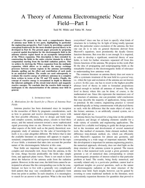
Consider the general radiation problem in Figure 1. We
assume that an arbitrary electric current J(r) exists inside a
volume V 0 enclosed by the surface S 0 . Let the antenna be
surrounded by an infinite, isotropic, and homogenous space
with electric permittivity ε and magnetic permeability µ. The

3
Fig. 1.
General description of antenna system.
antenna current will radiate electromagnetic fields everywhere
and we are concerned with the region outside the source
volume V 0 . We consider two characteristic regions. The first is
the region V enclosed by the spherical surface S and this will
be the setting for the near fields. The second region V ∞ is the
one enclosed by the spherical surface S ∞ taken at infinity and
it corresponds to the far fields. The complex Poynting theorem
states that [15]
∇ · S = − 1 2 J∗ · E + 2iω (w h − w e ) , (1)
where the complex Poynting vector is defined as S =
(1/2) E × H ∗ and the magnetic and electric energy densities
are given, respectively, by
w e = 1 4 εE · E∗ , w h = 1 4 µH · H∗ . (2)
Let us integrate (1) throughout the volume V
region.) We find
∫
ds 1 2 (E × H∗ ) = ∫ dv ( − 1 2 J∗ · E )
V 0
S
+2iω ∫ dv (w m − w e ) .
V
(near field
The divergence theorem was employed in writing the LHS
while the integral of the first term in the RHS was restricted to
the volume V 0 because the source current is vanishing outside
this region. The imaginary part of this equation yields
Im ∫ S ds 1 2 (E × H∗ ) = Im ∫ V 0
dv ( − 1 2 J∗ · E )
+2ω ∫ V dv (w (4)
h − w e ) .
The real part leads to
∫
Re ds 1 ∫
2 (E × H∗ ) = Re dv
V 0
S
(3)
(
− 1 )
2 J∗ · E . (5)
This equation stipulates that the real time-averaged power,
which is conventionally defined as the real part of the complex
Poynting vector, is given in terms of the work done by the
source on the field right at the antenna current. Moreover,
since this work is evaluated only over the volume V 0 , while
the surface S is chosen at arbitrary distance, we can see then
that the net time-averaged energy flux generated by the antenna
is the same throughout any closed surface as long as it does
enclose the source region V 0 . 1
We need to eliminate the source-field interaction (work)
term appearing in equation (3) in order to focus entirely on
the fields. To do this, consider the spherical surface S ∞ at
infinity. Applying the complex Poynting theorem there and
noticing that the far-field expressions give real power flow,
we conclude from (4) that
∫
Im dv
V 0
(
− 1 2 J∗ · E
)
∫
= −2ω dv (w h − w e ) .
V ∞
(6)
Substituting (6) into the near-field energy balance (4), we find
∫
Im ds 1 ∫
2 (E × H∗ ) = −2ω dv (w h − w e ) . (7)
S
V ∞−V
This equation suggests that the imaginary part of the complex
Poynting vector, when evaluated in the near field region, is
dependent on the difference between the electric and magnetic
energy in the region enclosed between the observation surface
S and the surface at infinity S ∞ , i.e., the total energy difference
outside the observation volume V . In other words, we
now know that the energy difference W h −W e is a convergent
quantity because the LHS of (7) is finite. 2 Since this condition
is going to play important role later, we stress it again as
∫
∣ dv (w h − w e )
∣ < ∞. (8)
V ∞ −V
Combining equations (5) and (7), we reach
∫
ds 1 ∫
2 (E × H∗ ) = P rad − 2iω dv (w h − w e ) , (9)
S
V ∞ −V
where the radiated energy is defined as
∫
P rad = Re ds 1 2 (E × H∗ ). (10)
S
We need to be careful about the interpretation of equation (9).
Strictly speaking, what this result tells us is only the following.
Form an observation sphere S at an arbitrary distance in the
near-field zone. As long as this sphere encloses the source
region V 0 , then the real part of the power flux, the surface
integral of the complex Poynting vector, will give the net
real power flow through S, while the imaginary part is the
total difference between the electric and magnetic energies
in the infinite region outside the observation volume V . We
repeat: the condition (8) is satisfied and this energy difference
is finite. Relation (9) is the theoretical basis for the traditional
expression of the antenna input impedance in terms of fields
surrounding the radiating structure [15], [6].
III. THE STRUCTURE OF THE ANTENNA NEAR FIELD IN
THE SPATIAL DOMAIN
We now turn to a closer examination of the nature of the
antenna near fields in the spatial domain, while the spectral
1 That is, the surface need not be spherical. However, in order to facilitate
actual calculations in later parts of this paper, we restrict ourselves to spherical
surfaces.
2 We remind the reader that all source singularises are assumed to be inside
the volume V 0 .

4
approach is deferred to Part II of this paper [9]. Here, we
consider the fields generated by the antenna that lying in the
intermediate zone, i.e., the interesting case between the far
zone kr → ∞ and the static zone kr → 0. The objective
is not to obtain a list of numbers describing the numerical
spatial variation of the fields away from the antenna, a task
well-achieved with present day computer packages. Instead,
we aim to attain a conceptual insight on the nature of the near
field by mapping out its inner structure in details. We suggest
that the natural way to achieve this is the use of the Wilcox
expansion [12]. Indeed, since our fields in the volume outside
the source region satisfy the homogenous Helmholtz equation,
we can expand the electric and magnetic fields as [12]
E (r) = eikr
r
∞∑
n=0
A n (θ, ϕ)
r n , H (r) = eikr
r
∞∑
n=0
B n (θ, ϕ)
r n ,
(11)
where A n and B n are vector angular functions dependent on
the far-field radiation pattern of the antenna and k = ω √ εµ
is the wavenumber. The far fields are the asymptotic limits of
the expansion. That is,
e
E (r) ∼
ikr
r→∞ r A e
0 (θ, ϕ) , H (r) ∼
ikr
r→∞ r B 0 (θ, ϕ) .
(12)
The reason why this approach is the convenient one can be
given in the following manner. We are interested in understanding
the structure of the near field of the antenna. In the
far zone, this structure is extremely simple; it is nothing but
the zeroth-order term of the Wilcox expansion as singled out
in (12). Now, as we leave the far zone and descend toward
the antenna current distribution, the fields start to get more
complicated. Mathematically speaking, this corresponds to the
addition of more terms into the Wilcox series. The implication
is that more terms (and hence the emerging complexity in
the spatial structure) are needed in order to converge to
accurate solution of the field as we get closer and closer to
the current distribution. Let us then divide the entire exterior
region surrounding the antenna into an infinite number of
spherical layers as shown in Figure 2. The outermost layer R 0
is identified with the far zone while the innermost layer R ∞ is
defined as the minimum sphere totally enclosing the antenna
current distribution. 3 In between these two regions, an infinite
number of layers exists, each corresponding to a term in the
Wilcox expansion as we now explain. The boundaries between
the various regions are not sharply defined, but taken only as
indicators in the asymptotic sense to be described momentarily.
4 The outermost region R 0 corresponds to the far zone.
The value of, say, the electric field there is A 0 exp (ikr)/r.
As we start to descend toward the antenna, we enter into
the next region R 1 , where the mathematical expression of
the far field given in (12) is no longer valid and has to be
augmented by the next term in the Wilcox expansion. Indeed,
we find that for r ∈ R 1 , the electric field takes (approximately,
3 Strictly speaking, there is no reason why R ∞ should be the minimum
sphere. Any sphere with larger size satisfying the mentioned condition will
do in theory.
4 To be precise, by definition only region R ∞ possesses a clear-cut boundary
(the minimum sphere enclosing the source distribution.)
Fig. 2.
General description of antenna near-field spatial structure.
asymptotically) the form A 0 exp (ikr) / r + A 1 exp (ikr) / r 2 .
Subtracting the two fields from each other, we obtain the
difference A 1 exp (ikr) / r 2 . Therefore, it appears to us very
natural to interpret the region R 1 as the “seat” of a field in
the form A 1 exp (ikr) / r 2 . Similarly, the nth region R n is
associated (in the asymptotic sense just sketched) with the
field form A n exp (ikr) / r n+1 . We immediately mention that
this individual form of the field does not satisfy Maxwell’s
equations. The nth field form given above is a mathematical
depiction of the effect of getting closer to the antenna on the
total (Maxwellian) field structure; it represents the contribution
added by the layer under consideration when passed through
by the observer while descending from the far zone to the
antenna current distribution. By dividing the exterior region in
this way, we become able to mentally visualize progressively
the various contributions to the total near field expression as
they are mapped out spatially. 5
It is important here to mention that, as will be proved in Part
II [9], localized and nonlocalized energies exist in each layer
in turn; that is, each region R n contains both propagating and
nonpropagating energies, which amounts to the observation
that in each region part of the field remains there, while the
remaining part of the field moves to the next larger layer. 6
What concerns us here (Part I) is not this more sophisticated
spectral analysis of the field associated with each layer, but
the simple mapping out of the antenna near fields into such
rough spatial distribution of concentric layers understood in
the asymptotic sense.
To be sure, this spatial picture, illuminating as it is, will
remain a mere definition unless it is corroborated by some
interesting consequences. This actually turns out to be the
case. As pointed out in the previous paragraph, it is possible to
show that certain theorems about the physical behavior of each
layer can be proved. Better still, it is possible to investigate
the issue of the mutual electromagnetic interaction between
different regions appearing in Figure 2. It turns out that a
5 It is for this reason that we refrain from rigourously defining the near field
as all the terms in the Wilcox expansion with n ≥ 1 as is the habit with some
writers. The reason is that such field is not Maxwellain.
6 The process is still even more complicated because of the interaction
(energy exchange) between the propagating and nonpropagating parts. See
[9] for analysis and conclusions.

5
general theorem (to be proved in Section V) can be established, where the mutual interaction between two angular vector fields
w h (r) = µ ∞∑ 〈B n , B n 〉
4 r 2n+2 + µ ∞∑ 〈B n , B n ′〉
2 r n+n′ +2 , (18) For example, in terms of this notation, the principle of reciprocity used
in deriving (15) and (16) can now be expressed economically in the form
n=0
n,n ′ 〈A
=0
n , A n ′〉 = 〈A n ′, A n 〉.
n>n ′ See Appendix A.
which shows that exactly “half” of these layers don’t electromagnetically
interact with each other. In order to understand
F and G is defined as 7
∫
the meaning of this remark, we need first to define precisely 〈F (θ, ϕ) , G (θ, ϕ)〉 ≡ dΩ Re {F (θ, ϕ) · G ∗ (θ, ϕ)}.
4π
what is expressed in the term ‘interaction.’ Let us use the
(19)
Wilcox expansion (11) to evaluate the electric and magnetic
energies appearing in (2). Since the series expansion under
consideration is absolutely convergent, and the conjugate of
an absolutely convergent series is still absolutely convergent,
the two expansions of E and E ∗ can be freely multiplied and
the resulting terms can be arranged as we please. The result
In deriving (17) and (18), we made use of the fact that the
energy series is uniformly convergent in θ and ϕ in order to
interchange the order of integration and summation. 8
Equations (17) and (18) clearly demonstrate the considerable
advantage gained by expressing the energy of the antenna
fields in terms of Wilcox expansion. The angular functional
is
w e = ε 4 E · E∗ = ε dependence of the energy density is completely removed by
∞∑ ∞∑ A n · A ∗ n ′
4 r n+n′ +2 , (13) integration over all the solid angles, and we are left afterwards
with a power expansion in 1/r, a result that provides direct
n=0 n ′ =0
intuitive understanding of the structure of the near field since
w h = µ 4 H · H∗ = µ ∞∑ ∞∑ B n · B ∗ n ′
4 r n+n′ +2 . (14) in such type of series more higher-order terms are needed for
accurate evaluation only when we get closer to the antenna
n=0 n ′ =0
body, i.e., for large 1/r. Moreover, the total energy is then
We rearrange the terms of these two series to produce the
following illuminating form
obtained by integrating over the remaining radial variable,
which is possible in closed form as we will see later in Section
w e (r) = ε ∞∑ A n · A ∗ n
4 r 2n+2 + ε ∞∑ Re {A n · A ∗ n ′} VI-B.
, (15) A particulary interesting observation, however, is that almost
2 r n+n′ +2
n=0
n,n ′ =0
“half” of the mutual interaction terms appearing in in (17)
n>n ′ and (18) are exactly zero. Indeed, we will prove later that if
w h (r) = µ ∞∑ B n · B ∗ n
4 r 2n+2 + µ ∞∑ Re {B n · B ∗ n ′} the integer n + n ′ is odd, then the interactions are identically
. (16) zero, i.e., 〈A
2 r n+n′ +2 n , A n ′〉 = 〈B n , B n ′〉 = 0 for n + n ′ = 2k + 1
n=0
n,n ′ =0
and k is integer. This represents, in our opinion, a significant
n>n ′ insight on the nature of antenna near fields in general. In order
In writing equations (15) and (16), we made use of the
reciprocity in which the energy transfer from layer n to layer
n ′ is equal to the corresponding one from layer n ′ to layer
n. The first sums in the RHS of (15) and (16) represent
the self interaction of the nth layer with itself. Those are
to prove this theorem and deduce other results, we need to
express the angular vector fields A n (θ, ϕ) and B n (θ, ϕ) in
terms of the antenna spherical TE and TM modes. This we
accomplish next by deriving the Wilcox expansion from the
multipole expansion.
the self interaction of the far field, the so-called radiation
density, and the self interactions of all the remanning (inner)
regions R n with n ≥ 1. The second sum in both equations
represents the interaction between different layers. Notice that
IV. DIRECT CONSTRUCTION OF THE ANTENNA
NEAR-FIELD STARTING FROM A GIVEN FAR-FIELD
RADIATION PATTERN
those interactions can be grouped into two categories, the
A. Introduction
interaction of the far field (0th layer in the Wilcox expansion)
with all other layers, and the remaining mutual interactions We have seen how the Wilcox expansion can be physically
between different layers before the far-field zone (again R interpreted as the mathematical embodiment of a spherical
n
with n ≥ 1.)
layering of the antenna exterior region understood in a convenient
asymptotic sense. The localization of the electromagnetic
Now because we are interested in the spatial structure of
near field, that is, the variation of the field as we move closer field within each of the regions appearing in Figure 2 suggests
to or farther from the antenna physical body where the current that the outermost region R 0 , the far zone, corresponds to the
distribution resides, it is natural to average over all the angular simplest field structure possible, while the fields associated
information contained in the energy expressions (15) and (16). with the regions close to the antenna exclusion sphere, R ∞ ,
That is, we introduce the radial energy density function of the are considerably more complex. However, as was pointed long
electromagnetic fields by integrating (15) and (16) over the ago, the entire field in the exterior region can be completely
entire solid angle Ω in order to obtain
determined recursively from the radiation pattern [12]. In this
section we further develop this idea by showing that the entire
w e (r) = ε ∞∑ 〈A n , A n 〉
4 r 2n+2 + ε ∞∑ 〈A n , A n ′〉
2 r n+n′ +2 , (17) region field can be determined from the far field directly, i.e.,
nonrecursively, by a simple construction based on the analysis
n=0
n,n ′ =0
n>n
of the far field into its spherical wavefunctions. In other words,
′

6
we show that a modal analysis of the radiation pattern, a
process that is computationally robust and straightforward,
can lead to complete knowledge of the exterior domain near
field, in an analytical form, as it is increasing in complexity
while progressing from the far zone to the near zone. This
description is meaningful because it has been expressed in
terms of physical radiation modes. The derivation will help to
appreciate the general nature of the near field spatial structure
that was given in Section III by gaining some insight into the
mechanism of electromagnetic coupling between the various
spatial regions defined in Figure 2, a task we address in details
in Section V.
B. Mathematical Description of the Far-Field Radiation Pattern
and the Concomitant Near-Field
Our point of departure is the far-field expressions (12),
where we observe that because A 0 (θ, ϕ) and B 0 (θ, ϕ) are
well-behaved angular vector fields tangential to the sphere,
it is possible to expand their functional variations in terms of
infinite sum of vector spherical harmonics [14], [15]. That is,
we write
∞∑ l∑
E (r) ∼
(−1) l+1 [a E (l, m) X lm
η eikr
r→∞ kr
l=0 m=−l
−a M (l, m) ˆr × X lm ] ,
(20)
∞∑ l∑
H (r) ∼
e ikr
r→∞ kr
(−1) l+1 [a M (l, m) X lm
l=0 m=−l
+a E (l, m) ˆr × X lm ] ,
(21)
the series being absolutely-uniformly convergent [13], [17].
Here, η = √ µ/ε is the wave impedance. a E (l, m) and
a M (l, m) stand for the coefficients of the expansion TE lm
and TM lm modes, respectively. 9 The definition of these modes
will be given in a moment. ( / The vector spherical harmonics
√l )
are defined as X lm = 1 (l + 1) LY lm (θ, ϕ), where
L = −i r × ∇ is the angular momentum operator; Y lm is the
spherical harmonics of degree l and order m defined as
√
(2l + 1) (l − m)!
Y lm (θ, ϕ) =
Pl m (cos θ) e imϕ , (22)
4π (l + m)!
where Pl
m stands for the associated Legendre function.
Since the asymptotic expansion of the spherical vector
wavefunctions is exact, 10 the electromagnetic fields throughout
the entire exterior region of the antenna problem can be
expanded as a series of complete set of of vector multipoles
[15]
E (r) = η ∞ ∑
l∑
l=0 m=−l
[
a E (l, m) h (1)
l
(kr) X lm
]
+ i k a M (l, m) ∇ × h (1)
l
(kr) X lm
,
(23)
9 These coefficients can also be determined from the antenna current
distribution, i.e., the source point of view. For derivations and discussion,
see [15].
10 That is, exact because of the expansion of the spherical Hankel function
given in (28.)
∑
H (r) = ∞ l∑ [
a M (l, m) h (1)
l
(kr) X lm
l=0 m=−l
]
− i k a E (l, m) ∇ × h (1)
l
(kr) X lm ,
(24)
which is absolutely and uniformly convergent. The spherical
Hankel function of the first kind h (1)
l
(kr) is used to model the
radial dependence of the outgoing wave in antenna systems. In
this formulation, we define the TE and TM modes as follows
⎧
⎨ r · H TE
lm
TE lm mode ≡ = a
⎩ E (l, m) l(l+1)
k
h (1)
l
(kr) Y lm (θ, ϕ) ,
r · E TE
lm = 0, (25)
⎧
⎨ r · E TE
lm
TM lm mode ≡ = a
⎩ M (l, m) l(l+1)
k
h (1)
l
(kr) Y lm (θ, ϕ) ,
r · H TE
lm = 0. (26)
Strictly speaking, the adjective ‘transverse’ in the labels TE
and TM is meaningless for the far field because there both
the electric and magnetic fields have zero radial components.
However, the terminology is still mathematically pertinent
because the two linearly independent angular vector fields
X lm and ˆr × X lm form complete set of basis functions for
the space of tangential vector fields on the sphere. For this
reason, and only for this, we still may frequently use phrases
like ‘far field TE and TM modes.’ In conclusion we find
that the far-field radiation pattern (20) and (21) determines
exactly the electromagnetic fields everywhere in the antenna
exterior region. This observation was corroborated by deriving
a recursive set of relations constructing the entire Wilcox
expansion starting only from the far field [12]. In the remaining
part of this section, we provide an alternative nonrecursive
derivation of the same result in terms of the far-field spherical
TE and TM modes. The upshot of our argument is the
unique determinability of the antenna near field in the various
spherical regions appearing in Figure 2 by a specified far
field taken as the starting point of the engineering analysis
of general radiating structures.
C. Derivation of the Exterior Domain Near-Field from the
Far-Field Radiation Pattern
The second terms in the RHS of (23) and (24) can be
simplified with the help of the following relation 11
∇ × h (1)
l
√
l(l+1)
r
h (1)
(kr) X lm = ˆri
[ l
(kr)
]
Y lm (θ, ϕ)
+ 1 ∂
r ∂r
rh (1)
l
(kr) ˆr × X lm (θ, ϕ) .
(27)
We expand the outgoing spherical Hankel function h (1)
l
(kr)
in a power series of 1/r using the following well-known series
[14],[18]
l∑
h (1)
l
(kr) = eikr b l n
r r n , (28)
n=0
11 Equation (27) can be readily derived from the definition of the operator
L = −i r × ∇ above and the expansion ∇ = ˆr (ˆr · ∇) −ˆr × ˆr × ∇, and by
making use of the relation L 2 Y lm = l (l + 1) Y lm .

7
where
b l n = (−i) l+1
i n
n!2 n k n+1 (l + n)!
(l − n)! . (29)
That is, in contrast to the situation with cylindrical wavefunctions,
the spherical Hankel function can be expanded only in
finite number of powers of 1/r, the highest power coinciding
with the order of the Hankel function l. Substituting (28) into
(27), we obtain after some manipulations
∇ × h (1)
l
X lm = i √ l (l + 1) eikr
r
l∑
− eikr
r
n=0
nb l n
r
ˆr × X n+1 lm + eikr
r
l∑
n=0
l∑
n=0
b l n
r n+1 ˆrY lm
ikb l n
r n ˆr × X lm .
(30)
By relabeling the indices in the summations appearing in
the RHS of (30) involving powers 1/r n+2 , the following is
obtained
∇ × h (1)
l
(kr) X lm = i √ l (l + 1) eikr
r
− eikr
r
l+1 ∑
n=1
(n−1)b l n−1
r n
ˆr × X lm + eikr
r
l+1 ∑
n=1
l∑
n=0
b l n−1
r
ˆrY n lm
ik bl n
r n ˆr × X lm .
(31)
Now it will be convenient to write this expression in the
following succinct form
where
and
∇ × h (1)
l
X lm = eikr
r
c l n =
∑l+1
n=0
c l n ˆrY lm + d l n ˆr × X lm
r n , (32)
{ 0, n = 0,
i √ l (l + 1)b l n−1, 1 ≤ n ≤ l + 1.
(33)
⎧
⎨ ikb l 0, n = 0,
d l n = ikb l n − (n − 1) b l
⎩
n−1, 1 ≤ n ≤ l, (34)
−lb l l , n = l + 1.
Using (32), the expansions (23) and (24) can be rewritten as
E (r) = η ∞ ∑
H (r) = ∞ ∑
l∑
l=0 m=−l
+ i k a M (l, m) eikr
r
l∑
l=0 m=−l
− i k a E (l, m) eikr
r
[
a E (l, m) eikr
r
l+1 ∑
g l n X lm
r n
l+1 ∑
n=0
c l n ˆrY lm+d l n ˆr×X lm
]
n=0
r n
[
a M (l, m) eikr
r
l+1 ∑
g l n X lm
r n
l+1 ∑
n=0
c l n ˆrY lm+d l n ˆr×X lm
]
n=0
r n
,
,
(35)
(36)
Assuming that the electromagnetic field in the antenna
exterior region is well-behaved, it can be shown that the
infinite double series in (35) and (36) involving the l- and
n- sums are absolutely convergent, and subsequently invariant
to any permutation (rearrangement) of terms [16]. Now let us
consider the first series in the RHS of (36). We can easily
see that each power r −n will arise from contributions coming
from all the multipoles of degree l ≥ n. That is, we rearrange
as
∞∑ l∑
l∑
a M (l, m) eikr b l n
r r
X n lm
l=0 m=−l
n=0
∞∑ ∞∑ l∑
= eikr
r
n=0
1
r n
l=n m=−l
a M (l, m) b l nX lm .
(37)
The situation is different with the second series in the RHS of
(36). In this case, contributions to the 0th and 1st powers
of 1/r originate from the same multipole, that of degree
l = 0. Afterwards, all higher power of 1/r, i.e., terms with
n ≥ 2, will receive contributions from multipoles of the
(n − 1)th degree, but yet with different weighting coefficients.
We unpack this observation by writing
∞∑
l∑
l=0 m=−l
= − eikr
ikr
+ ∞ ∑
n=1
i
k a E (l, m) eikr
r
[
∞∑ l∑
1
r n
l=0 m=−l
∞∑
l∑
l=n−1 m=−l
l+1 ∑
n=0
(c l n ˆrY lm+d l n ˆr×X lm)
r n
a E (l, m) ( c l 0 ˆrY lm + d l 0 ˆr × X lm
)
a E (l, m) ( c l n ˆrY lm + d l n ˆr × X lm
) ] ,
(38)
That is, from (37) and (38) equation (36) takes the form
∞∑
H (r) = eikr B n (θ, ϕ)
r r n , (39)
where
B 0 (θ, ϕ) = ∞ ∑
B n (θ, ϕ) = ∞ ∑
−
∞ ∑
l∑
l=n−1 m=−l
l∑
l=0 m=−l
l∑
l=n m=−l
ia E (l,m)
k
n=0
(−i) l+1
k
[a M (l, m) X lm
+a E (l, m) ˆr × X lm ] ,
a M (l, m) b l nX lm
(
c
l
n ˆrY lm + d l n ˆr × X lm
)
, n ≥ 1.
(40)
(41)
By exactly the same procedure, we derive from equation (35)
the following result
where
A 0 (θ, ϕ) = η ∞ ∑
A n (θ, ϕ) = η ∞ ∑
+η
∞∑
l∑
l=n−1 m=−l
E (r) = eikr
r
l∑
l=0 m=−l
l∑
l=n m=−l
ia M (l,m)
k
∞∑
n=0
(−i) l+1
k
A n (θ, ϕ)
r n , (42)
[a E (l, m) X lm
−a M (l, m) ˆr × X lm ] ,
a E (l, m) b l nX lm
(43)
(
c
l
n ˆrY lm + d l n ˆr × X lm
)
, n ≥ 1.
(44)
Therefore, the Wilcox series is derived from the multipole
expansion and the exact variation of the angular vector fields
A n and B n are directly determined in terms of the spherical
far-field modes of the antenna. We notice that these two
nth vector fields take the form of infinite series of spherical

8
harmonics of degrees l ≥ n, i.e., the form of the tail
of the infinite series appearing in the far field expression
(20) and (21). The coefficients, however, of the same modes
appearing in the latter series are now modified by the simple n-
dependence of c l n and d l n as given in (33) and (34). Conversely,
the contribution of each l-multipole to the respective terms in
the Wilcox expansion is determined by the weights c l n and d l n,
which are varying with l. There is no dependence on m in this
derivation of the Wilcox terms in terms of the electromagnetic
field multipoles.
D. General Remarks
As can be seen from the direct relations (43), (44), (40), and
(41), the antenna near field in the various regions R n defined in
Figure 2 is developable in a series of higher-order TE and TM
modes, those modes being uniquely determined by the content
of the far-field radiation pattern. Some observations on this
derivation are worthy mention. We start by noticing that the
expressions of the far field (43) and (40), the initial stage of
the analysis, are not homogenous with the expressions of the
inner regions (44) and (41). This can be attributed to mixing
between two adjacent regions. Indeed, in the scalar problem
only modes of order l ≥ n contribute to the content of the
region R n . However, due to the effect of radial differentiation
in the second term of the RHS of (27), the aforementioned
mixing between two adjacent regions emerges to the scene,
manifesting itself in the appearance of contributions from
modes with order n − 1 in the region R n . This, however,
always comes from the dual polarization. For example, in the
magnetic field, the TM lm modes with l ≥ n contribute to
the field localized in region R n , while the contribution of the
TE lm modes comes from order l ≥ n − 1. The dual statement
holds for the electric field. As will be seen in Section V, this
will lead to similar conclusion for electromagnetic interactions
between the various regions.
We also bring to the reader’s attention the fact that the
derivation presented in this section does not imply that the
radiation pattern determines the antenna itself, if by the
antenna we understand the current distribution inside the
innermost region R ∞ . There is an infinite number of current
distributions that can produce the same far-field pattern. Our
results indicate, however, that the entire field in the exterior
region, i.e., outside the region R ∞ , is determined exactly and
nonrecursively by the far field. We believe that the advantage
of this observation is considerable for the engineering study of
electromagnetic radiation. Antenna designers usually specify
the goals of their devices in terms of radiation pattern characteristics
like sidelobe level, directivity, cross polarization,
null location, etc. It appears from our analysis that an exact
analytical relation between the near field and these design
goals do exist in the form derived above. Since the engineer
can still choose any type of antenna that fits within the enclosing
region R ∞ , the results of this paper should be viewed
as a kind of canonical machinery for generating fundamental
relations between the far-field performance and the lower
bound formed by the field behavior in the entire exterior
region compatible with any antenna current distribution that
can be enclosed inside R ∞ . For example, relations (69) and
(70) provide the exact analytical form for the reactive energy
in the exterior region. This then forms a lower bound on the
actual reactive energy for a specific antenna, because the field
inside R ∞ will only add to the reactive energy calculated
for the exterior region. To summarize this important point,
our results in this paper apply only to a class 12 of antennas
compatible with a given radiation pattern, not to a particular
antenna current distribution. 13 This, we repeat, is a natural
theoretical framework for the engineering analysis of antenna
fundamental performance measures. 14
V. A CLOSER LOOK AT THE SPATIAL DISTRIBUTION OF
ELECTROMAGNETIC ENERGY IN THE ANTENNA EXTERIOR
A. Introduction
REGION
In this section, we utilize the results obtained in Section
IV in order to evaluate and analyze the energy content of the
antenna near field in the spatial domain. We continue to work
within the overall picture sketched in Section III in which the
antenna exterior domain was divided into spherical regions
understood in the asymptotic sense (Figure 2), and the total
energy viewed as the sum of self and mutual interactions of
among these regions. Indeed, we will treat now in details
the various types of interactions giving rise to the radial
energy density function in the form introduced in (17) and
(18). The calculation will make use of the following standard
orthogonality relations
∫
4π dΩ X lm · X ∗ l ′ m = δ ′ ll ′δ mm ′,
∫
4π dΩ X lm · (ˆr × X ∗ l ′ m ′) = 0,
∫
(45)
4π dΩ (ˆr × X lm) · (ˆr × X ∗ l ′ m ′) = δ ll ′δ mm ′,
ˆr · (ˆr × X lm ) = ˆr · X lm = 0,
where δ lm stands for the Kronecker delta function.
B. Self Interaction of the Outermost Region (Far Zone, Radiation
Density)
The first type of terms is the self interaction of the fields
in region R 0 , i.e., the far zone. These are due to the terms
involving 〈A 0 , A 0 〉 and 〈B 0 , B 0 〉 for the electric and magnetic
fields, respectively. From (19), (43), (40), and (45), we readily
obtain the familiar expressions
〈A 0 , A 0 〉 = η2
k 2
∞ ∑
l∑
l=0 m=−l
[
|a E (l, m)| 2 + |a M (l, m)| 2] ,
(46)
12 Potentially infinite in size.
13 This program will be studied thoroughly in [11].
14 The extensively-researched area of fundamental limitations of electrically
small antennas is a special case in this general study. We don’t presuppose
any restriction on the size of the innermost region R ∞, which is required only
to enclose the entire antenna in order for the various series expansions used in
this paper to converge nicely. Strictly speaking, electrically small antennas are
more challenging for the impedance matching problem than the field point of
view. The field structure of an electrically small antenna approaches the field
of an infinitesimal dipole and hence does not motivate the more sophisticated
treatment developed in this paper, particulary the spectral approach of Part II.

9
〈B 0 , B 0 〉 = 1 k 2 ∞ ∑
l∑
l=0 m=−l
[
|a M (l, m)| 2 + |a E (l, m)| 2] .
(47)
That is, all TE lm and TM lm modes contribute to the self
interaction of the far field. As we will see immediately, the
picture is different for the self interactions of the inner regions.
C. Self Interactions of the Inner Regions
From (19), (44), and (45), we obtain
〈A n , A n 〉 = η 2 ∑ ∞ l∑ ∣ ∣
∣a E (l, m) b l n
+ η2
k 2
∞∑
l=n−1 m=−l
l=n m=−l
l∑
( |a M (l, m)| 2 ∣ c l ∣ 2 n + ∣ ∣d l ∣ 2) n , n ≥ 1,
Similarly, from (19), (41), and (45) we find
∑
〈B n , B n 〉 = ∞ l∑ ∣
∣a M (l, m) b l ∣ 2
n
+ 1
k 2
∞∑
l=n m=−l
l∑
l=n−1 m=−l
( |a E (l, m)| 2 ∣ c l ∣ 2 n + ∣ ∣d l ∣ 2) n , n ≥ 1.
∣ 2
(48)
(49)
Therefore, in contrast to the case with the radiation density,
the 0th region, the self interaction of the nth inner region
(n > 0) consists of two types: the contribution of TE lm modes
to the electric energy density, which involves only modes with
l ≥ n; and the contribution of the TM lm modes to the same
energy density, which comes this time from modes with order
l ≥ n − 1. The dual situation holds for the magnetic energy
density. This qualitative splitting of the modal contribution to
the energy density into two distinct types is ultimately due to
the vectorial structure of Maxwell’s equations. 15
D. Mutual Interaction Between the Outermost Region and The
Inner Regions
We turn now to the mutual interactions between two different
regions, i.e., to an examination of the second sums in the
RHS of (17) and (18). We first evaluate here the interaction
between the far field and an inner region with index n. From
(19), (43), (44), and (45), we compute
〈A 0 , A n 〉 = η2
k
+ η2
k 2
∞∑
l∑
l=n m=−l
∞∑
l∑
l=n−1 m=−l
g 1 n (l, m) |a E (l, m)| 2
g 2 n (l, m) |a M (l, m)| 2 , n ≥ 1.
From (19), (40), (41), and (45), we also reach to
∞∑ l∑
〈B 0 , B n 〉 = 1 k
gn 1 (l, m) |a M (l, m)| 2
+ 1
k 2
l=n m=−l
∞∑
l∑
l=n−1 m=−l
From (29), we calculate
{ }
gn 1 (l, m) ≡ Re (−i) l+1 b l∗
n =
15 Cf. Section IV-D.
g 2 n (l, m) |a E (l, m)| 2 , n ≥ 1.
(50)
(51)
{
0, n odd,
(−1) 3n/2
n!2 n k n+1 (l+n)!
(l−n)! , n even.
(52)
Similarly, we use (34) to calculate
{ }
gn 2 (l, m) ≡ Re (−i) l+1 id l∗
n
{ kg
1
= n (l, m) − (n − 1) gn 3 (l, m) , 1 ≤ n ≤ l,
−lgl+1 3 (l, m) , n = l + 1. (53)
Here, we define
g 3 n (l, m) ≡
{
0, n odd,
(−1) 3n/2−1
(n−1)!2 n−1 k n (l+n−1)!
(l−n−1)! , n even. (54)
Therefore, it follows that the interaction between the far field
zone and any inner region R n , with odd index n is exactly
zero. This surprising result means that “half” of the mutual
interactions between the regions comprising the core of the
antenna near field on one side, and the far field on the other
side, is exactly zero. Moreover, the non-zero interactions, i.e.,
when n is even, are evaluated exactly in simple analytical
form. We also notice that this nonzero interaction with the nth
region R n involves only TM lm and TE lm modes with l ≥ n
and l ≥ n − 1. The appearance of terms with l = n − 1 is
again due to the polarization structure of the radiation field. 16
E. Mutual Interactions Between Different Inner Regions
We continue the examination of the mutual interactions
appearing in the second term of the RHS of (17) and (18),
but this time we focus on mutual interactions of only inner
regions, i.e., interaction between region R n and R n ′ where
both n ≥ 1 and n ′ ≥ 1. From (19), (44), and (45), we arrive
to
∞∑ l∑
〈A n , A n ′〉 = η 2 gn,n 4 (l, m) |a ′ E (l, m)| 2
+ η2
k 2
+ η2
k 2
∞∑
l=ϑ n′ −1
n−1
l=ϑ n′ n
∞∑
m=−l
l∑
l=ϑ m n m=−l
l∑
m=−l
g 5 n,n ′ (l, m) |a M (l, m)| 2
g 6 n,n ′ (l, m) |a M (l, m)| 2 , n, n ′ ≥ 1.
Similarly, from (19), (41), and (45), we reach to
〈B n , B n ′〉 = ∞ ∑
+ 1
k 2
+ 1
k 2
∞∑
l=ϑ n′ −1
n−1
l=ϑ n′
n
∞∑
l=ϑ n′ −1
n−1
l∑
m=−l
l∑
m=−l
l∑
m=−l
g 4 n,n ′ (l, m) |a M (l, m)| 2
g 5 n,n ′ (l, m) |a E (l, m)| 2
g 6 n,n ′ (l, m) |a E (l, m)| 2 , n, n ′ ≥ 1.
(55)
(56)
Here we define ϑ m n ≡ max (n, m). Finally, formulas for gn,n 4 ′,
gn,n 5 ′, and g6 n,n ′ are derived in Appendix B.
Now, it is easy to see that if n + n ′ is even (odd), then
n − 1 + n ′ − 1 is also even (odd). Therefore, we conclude
from the above and Appendix B that the mutual interaction
between two inner regions R n and R n ′ is exactly zero if
n + n ′ is odd. For the case when the interaction is not
zero, the result is evaluated in simple analytical form. This
16 Cf. Section IV-D.

10
nonzero term involves only TM lm and TE lm modes with
l ≥ max(n, n ′ ) and l ≥ max(n − 1, n − 1 ′ ). Therefore, there
exists modes satisfying min(n, n ′ ) ≤ l < max(n, n ′ ) and
min(n−1, n ′ −1) ≤ l < max(n−1, n−1 ′ ) that simply do not
contribute to the electromagnetic interaction between regions
R n and R n ′. The appearance of terms with l = n−1 is again a
consequence of coupling through different modal polarization
in the electromagnetic field under consideration. 17
F. Summary and Conclusion
In this Section, we managed to express all the interaction
integrals appearing in the general expression of the antenna
radial energy density (17) and (18) in the exterior region in
closed analytical form involving only the TM lm and TE lm
modes excitation amplitudes a M (l, m) and a E (l, m). The
results turned out to be intuitive and comprehensible if the
entire space of the exterior region is divided into spherical
regions understood in the asymptotic sense as shown in
Figure 2. In this case, the radial energy densities (17) and
(18) are simple power series in 1/r, where the amplitude
of each term is nothing but the mutual interaction between
two regions. From the basic behavior of such expansions, we
now see that the closer we approach the exclusion sphere that
directly encloses the antenna current distribution, i.e., what
we called region R ∞ , the more terms we need to include in
the energy density series. However, the logic of constructing
those higher-order terms clearly shows that only higher-order
far-field modes enter into the formation of such increasing
powers of 1/r, confirming the intuitive fact that the complexity
of the near field is an expression of richer modal content
where more (higher-order) modes are needed in order to
describe the intricate details of electromagnetic field spatial
variation. As a bonus we also find that the complex behavior
of the near field, i.e., that associated with higher-order farfield
modes, is localized in the regions closer to the antenna
current distribution, so in general the nearer the observation to
the limit region R ∞ , the more complex becomes the near-field
spatial variation.
Finally. it is interesting to note that almost “half” of the
interactions giving rise to the amplitudes of the radial energy
density series (17) and (18) are exactly zero— i.e., the
interactions between regions R n and R ′ n when n + n ′ is odd.
There is no immediate apriori reason why this should be the
case or even obvious, the logic of the verification presented
here being after all essentially computational. We believe that
further theoretical research is needed to shed light on this
conclusion from the conceptual point of view, not merely the
computational one.
VI. THE CONCEPT OF REACTIVE ENERGY: THE CIRCUIT
POINT OF VIEW OF ANTENNA SYSTEMS
A. Introduction
In the common literature on antennas, the relation (9) has
been taken as an indication that the so-called ‘reactive’ field
is responsible of the imaginary part of the complex Poynting
17 Cf. Section IV-D.
vector. Since it is this term that enters into the imaginary
part of the input impedance of the antenna system, and since
from circuit theory we usually associate the energy stored
in the circuit with the imaginary part of the impedance, a
trend developed in regarding the convergent integral (7) as an
expression of the energy ‘stored’ in the antenna’s surrounding
fields, and even sometimes call it ‘evanescent field.’ Hence,
there is a confusion resulting from the uncritical use of the
formula: reactive energy = stored energy = evanescent energy.
However, there is nothing in (9) that speaks about such
profound conclusion! The equation, read at its face value, is an
energy balance derived based on certain convenient definitions
of time-averaged energy and power densities. The fact that
the integral of the energy difference appears as the imaginary
part of the complex Poynting vector is quite accidental and
relates to the contingent utilization of time-harmonic excitation
condition. However, the concepts of stored and evanescent
field are, first of all, spatial concepts, and, secondly, are
thematically broad; rightly put, these concepts are fundamental
to the field point of view of general antenna systems. The
conclusion that the stored energy is the sole contributor to the
reactive part of the input impedance of the antenna system
is an exaggeration of the circuit model that was originally
advanced to study the antenna through its input port. The field
structure of the antenna is richer and more involved than the
limited ‘terminal-like’ point of view implied by circuit theory.
The concept of reactance is not isomorphic to neither stored
nor evanescent energy.
In this section, we will first carefully construct the conventional
reactive energy and show that its natural definition
emerges only after the use of the Wilcox expansion in writing
the radiated electromagnetic fields. In particular, we show that
the general theorem we proved above about the null result of
the interaction between the far field and inner layers with odd
index is one of the main reasons why a finite reactive energy
throughout the entire exterior region is possible. Moreover, we
show that such reactive energy is evaluated directly in closed
form and that no numerical infinite integral is involved in its
computation. We then end this section be demonstrating the
existence of certain ambiguity in the achieved definition of
the reactive energy when attempts to extend its use beyond
the circuit model of the antenna system are made.
B. Construction of the Reactive Energy Densities
We will call any energy density calculated with the point of
view of those quantities appearing in the imaginary part of (9)
reactive densities. 18 When someone tries to calculate the total
electromagnetic energies in the region V ∞ − V , the result is
divergent integrals. In general, we have
∫
dv (w h + w e ) = ∞. (57)
V ∞ −V
However, condition (8) clearly suggests that there is a common
term between w e and w h which is the source of the trouble
18 The question of the reactive field is usually ignored in literature under
the claim of having difficulty treating the cross terms [2].

11
in calculating the total energy of the antenna system. We
postulate then that
w e ≡ w 1 e + w rad , w h ≡ w 1 h + w rad . (58)
Here we
1 and wh 1 are taken as reactive energy densities we
hope to prove them to be finite. The common term w rad is
divergent in the sense
∫
dvw rad = ∞. (59)
V ∞−V
Therefore, it is obvious that w h −w e = wh 1 −w1 e, and therefore
we conclude from (8) that
∫
∣ dv ( wm 1 − we) ∣ 1 ∣∣ < ∞. (60)
V ∞−V
Next, we observe that the asymptotic analysis of the complex
Poynting theorem allows us to predict that the energy difference
w h − w e approaches zero in the far-field zone. This is
consistent with (58) only if we assume that
w h (r) ∼ w rad (r) , w e (r) ∼ w rad (r) . (61)
r→∞ r→∞
That is, in the asymptotic limit r → ∞, the postulated
quantities wh,e
1 can be neglected in comparison with w rad.
In other words, the common term w rad is easily identified as
the radiation density at the far-field zone. 19 It is well-known
that the integral of this density is not convergent and hence
our assumption in (59) is confirmed. Moreover, this choice for
the common term in (58) has the merit of making the energy
difference, the imaginary part of (9), “devoid of radiation,” and
hence the common belief in the indistinguishability between
the reactive energy and the stored energy. As we will show
later, this conclusion cannot be correct, at least not in terms
of field concepts.
The final step consists in showing that the total energy is
finite. Writing the appropriate sum with the help of (58), we
find
Wh 1 + W e 1 ≡ ∫ V ∞ −V dv ( wh 1 + )
∫
w1 e
= lim r ′ →∞ V (r ′ )−V dv [w h (r) + w e (r) − 2w rad ] .
(62)
To prove that this integral is finite, we make use of the Wilcox
expansion of the vectorial wavefunction. First, we notice that
the far-field radiation patterns are related to each others by
B 0 (θ, ϕ) = (1/η)ˆr × A 0 (θ, ϕ) , (63)
This relation is the origin of the equality of the radiation
density of the electric and magnetic types when evaluated in
the far-field zone. That is, we have
w rad (r) = (ε/4)(A 0 · A ∗ 0)/r 2 = (µ/4)(B 0 · B ∗ 0)/r 2 . (64)
Employing the expansion (11) in the energy densities (2), it
is found that
w e (r) = w rad (r) + ε 〈A 0,A 1〉
2 r
∞∑
3
+ ε 4
n=1
〈A n ,A n 〉
r 2n+2 + ε 2
∞∑
r n+n′ +2
, (65)
〈A n ,A n ′ 〉
n,n ′ =1
n>n ′
19 As will be seen shortly, it is meaningless to speak of a radiation density
in the near-field zone.
w h (r) = w rad (r) + µ 2
∞∑
+ µ 4
n=1
〈B 0 ,B 1 〉
r 3
〈B n,B n〉
r 2n+2 + µ 2
∞∑
r n+n′ +2
. (66)
〈B n ,B n ′ 〉
n,n ′ =1
n>n ′
By carefully examining the radial behavior of the total energies,
we notice that the divergence of their volume integral
over the exterior region arises from two types of terms:
1) The first type is that associated with the radiation density
w rad , which takes a functional form like 〈A 0 , A 0 〉 / r 2
and 〈B 0 , B 0 〉 / r 2 . The volume integral of such terms
will give rise to linearly divergent energy.
2) The second type is that associated with functional forms
like 〈A 0 , A 1 〉 / r 3 and 〈B 0 , B 1 〉 / r 3 . The volume integral
of these terms will result in energy contribution that is
logarithmically divergent.
However, we make use of the fact proved in Section V-D
stating that the interactions 〈A 0 , A 1 〉 and 〈B 0 , B 1 〉 are identically
zero. Therefore, only singularities of the first type will
contribute to the total energy. Making use of the equality (64)
and the definitions (58), those remaining singularities can be
eliminated and we are then justified in reaching the following
series expansions for the reactive radial energy densities
w 1 e (r) = ε 4
w 1 h (r) = µ 4
∞∑
n=1
∞∑
n=1
〈A n , A n 〉
r 2n+2 + ε 2
〈B n , B n 〉
r 2n+2 + µ 2
∞∑
n,n ′ =1
〈A n , A n ′〉
r n+n′ +2 , (67)
n>n ′
∞∑
n,n ′ =1
〈B n , B n ′〉
r n+n′ +2 . (68)
n>n ′
For the purpose of demonstration, let us take a hypothetical
spherical surface that encloses the source region V 0 . Denote
by a the radius of smallest such sphere, i.e., R ∞ = {(r, θ, ϕ) :
r ≤ a}. The evaluation of the total reactive energy proceeds
then in the following way. The expansions (67) and (68) are
uniformly convergent in r and therefore we can interchange the
order of summation and integration in (62). After integrating
the resulting series term by term, we finally arrive to the
following results
W 1 e =
W 1 h =
∞∑
n=1
∞∑
n=1
(ε/4) 〈A n , A n 〉
∞
(2n − 1) a 2n−1 + ∑ (ε/2) 〈A n , A n ′〉
(n + n ′ − 1) a n+n′ −1 ,
n,n ′ =1
n>n ′
(µ/4) 〈B n , B n 〉
∞
(2n − 1) a 2n−1 + ∑
(69)
(µ/2) 〈B n , B n ′〉
(n + n ′ − 1) a n+n′ −1 .
n,n ′ =1
n>n ′
(70)
Therefore, the total reactive energy is finite. It follows then
that the definitions postulated above for the reactive energy
densities w 1 h and w1 e are consistent. Moreover, from the results
of Section V, we now see that total reactive energies (69)
and (70) are evaluated completely in analytical form and that
in principle no computation of infinite numerical integrals is
needed here. 20
20 Special cases of (69) and (70) appeared throughout literature. For example,
see [2], [3], [5], [6].

12
We stress here that the contribution of the expressions (69)
and (70) is not merely having at hand a means to calculate the
reactive energy of the antenna. The main insight here is the fact
that the same formulas contain information about the mutual
dependence of 1) the quality factor Q (through the reactive
energy), 2) the size of the antenna (through the dependence on
a), and 3) the far-field radiation pattern (through the interaction
terms and the results of Section V.) The derivation above
points to the relational structure of the antenna from the
engineering point of view in the sense that the quantitative
and qualitative interrelations of performance measures like
directivity and polarization (far field), matching bandwidth
(the quality factor), and the size become all united within
one look. 21 The being of the antenna is not understood by
computing few numbers, but rather by the interconnection of
all measures within an integral whole. The relational structure
of the antenna system will be further developed with increasing
sophistication in [9] and [10].
C. The Ambiguity of the Concept of Reactive Field Energy
It is often argued in literature that the procedure outlined
here is a “derivation” of the energy ‘stored’ in antenna systems.
Unfortunately, this matter is questionable. The confusion arises
from the bold interpretation of the term w rad as a radiation
energy density everywhere. This cannot be true for the following
reason. When we write w rad = (ε/4)E rad · E ∗ rad =
(µ/4)H rad·H ∗ rad
, the resulted quantity is function of the radial
distance r. However, the expression loses its meaning when
the observation is at the near-field zone. Indeed, if one applies
the complex Poynting theorem there, he still gets the same
value of the net real power flow, but the whole field expression
must now be taken into account, not just the far-field terms.
Such field terms, whose amplitudes squared were used to
calculate w rad , simply don’t satisfy Maxwell’s equations in
the near-field zone. For this reason, it is incoherent to state
that “since energy is summable quantity, then we can split the
total energy into radiation density and non-radiation density”
as we already did in (58). These two equations are definitions
for the quantities wh 1 and w1 e, not derivations of them by a
physical argument. 22
To make this argument transparent, let us imagine the
following scenario. Scientist X has already gone through
all the steps of the previous procedure and ended up with
mathematically sound definitions for the quantities wh
1 and
we, 1 which he duped reactive energy densities. Now, another
person, say Scientist Y, is trying to solve the same problem.
However, for some reason he does not hit directly on the term
w rad found by Scientist X, but instead considers the positive
term Υ appearing in the equation
w rad = α + Υ, (71)
21 Extensive numerical analysis of the content of (69) and (70) will be
carried out elsewhere [11].
22 One has always to remember that the concept of energy in electromagnetism
is not straightforward. All energy relations must be viewed as rigorous
mathematical propositions derived from the calculus of Maxwell’s equations,
and afterwards interpreted as energies and power in the usual mechanical
sense.
where we assume
and
∫
∣ ∣∣∣
∫
V ∞−V
V ∞−V
dvΥ = ∞ (72)
dvα
∣ < ∞. (73)
That is, the divergent density w rad is composed of two terms,
one convergent and the other divergent. We further require that
w rad (r) = α (r) + Υ (r) ∼ Υ (r) . (74)
r→∞
That is, the asymptotic behavior of w rad is dominated by the
term Υ. The equations of the total energy density now become
and
where
w e = w 1 e + w rad = ( w 1 e + α ) + Υ = w 2 e + Υ (75)
w h = w 1 h + w rad = ( w 1 h + α ) + Υ = w 2 h + Υ, (76)
w 2 e = w 1 e + α, w 2 h = w 1 h + α. (77)
Now, it is easily seen that the conditions required for the
“derivation” of w 1 h and w1 e are already satisfied for the new
quantities w 2 h and w2 e. That is, we have
w h,e (r) = wh,e 1 (r) + α (r) + Υ (r) ∼ Υ (r)
r→∞
∼ w rad (r) ,
r→∞
(78)
which states that the large argument approximation of Υ(r)
coincides with the radiation density w rad (r) at the far-field
zone. Furthermore, it is obvious that
∫
V dv (w ∞−V h − w e ) = ∫ V dv ( ∞−V
wh 1 − )
w1 e
= ∫ V ∞ −V dv ( wh 2 − ) (79)
w2 e ,
and hence is convergent. Also,
∫
V dv ( ∞−V
wh 2 + )
w2 e
= ∫ V ∞ −V dv [(w h − w e ) − 2w rad ] − 2 ∫ V ∞ −V dvα (80)
and hence is also convergent. Therefore, the quantities w 2 h
and w 2 e will be identified by Scientist Y as legitimate ‘stored’
energy in his quest for calculating the reactive energy density
of the antenna. This clearly shows that the reactive energy
calculated this way cannot be a legitimate physical quantity in
the sense that it is not unique. In our opinion, the procedure of
computing the reactive energy is artificial since it is tailored to
fit an artificial requirement, the engineering circuit description
of the antenna port impedance. Subtracting the radiation
energy from the total energy is not a unique recipe of removing
infinities. As should be clear by now, nobody seems to have
thought that maybe the subtracted term w rad itself contains a
non-divergent term that is part of a physically genuine stored
energy density defined through a non-circuit approach, i.e.,
field formalism per se. 23
23 In Part II [9], we will show explicitly that this is indeed the case.

13
D. Critical Reexamination of the Near-Field Shell
We turn now to a qualitative and quantitative analysis of
the magnitude of the ambiguity in the identification of the
stored energy with the reactive energy. Let a be the minimum
size of the hypothetical sphere enclosing the source region V 0 .
Denote by b the radial distance b > a at which the term w rad
dominates asymptotically the reactive energy densities w 1 h and
w 1 e. It is the contribution of w rad to the energy density lying
in the interval a < r < b which is ambiguous in the sense that
it can be arbitrarily decomposed into the sum of two positive
functions α(r) + Υ(r) in the indicated interval. However, if
the total contribution of the splitable energy density within this
interval is small compared with the overall contributions of the
higher-order terms, then the ambiguity in the definition of the
reactive energy densities does not lead to serious problems in
practice. The evaluation of all the integrals with respect to r
gives an expression in the form 24
We 1 + We 1 = ( ε
4 〈A 0, A 0 〉 + µ 4 〈B 0, B 0 〉 ) (b − a)
∑
+ ∞ ∞∑
(
n=1 n ′ =1
ε〈A n ,A n ′ 〉+µ〈B n ,B n 〉
4(n+n ′ −1)
1
a n+n′ −1
−
1
b n+n′ −1
(81)
The integration with respect to the solid angle yields quantities
with the same order of magnitude. Therefore, we focus in
our qualitative examination on the radial dependance. It is
clear that when a becomes very small, i.e., a ≪ 1, the
higher-order terms dominate the sum and the contribution
of the lowest-order term can be safely neglected, with all
its ambiguities. On the other hand, when a approaches the
antenna operating wavelength and beyond, the higher-order
terms rapidly decay and the lowest-order term dominates the
contribution to the total energy in the interval a < r < b.
Since it is in this very interval that we find the ambiguity
in defining the reactive energy, we conclude that the reactive
energy as defined in circuit theory cannot correspond to a
physically meaningful definition of ‘stored’ field energy, and
that the results calculated in literature as fundamental limit
to antenna Q are incoherent when the electrical size of the
exclusion volume approaches unity and beyond.
One more point that need to be examined in the above
argument relates to the choice of b. Of course, b cannot be
fixed arbitrarily because it is related to the behavior of the
higher-order terms, i.e., b is the radius of the radiation sphere,
the sphere through which most of the field is converted into
radiation field. 25 Therefore, in our argument above a reaches
the critical value of unit wavelength but cannot increase
significantly because it is bounded from above by b, which
is not freely varying like a. The upshot of the argument
is that the vagueness in the precise value of b is nothing
but the vagueness in any asymptotic expansion in general
where accuracy is closely tied to the physical conditions of
the particular situation under consideration. In this situation,
24 In writing (81), we explicitly dropped the zero terms involving 〈A 0 , A 1 〉
and 〈B 0 , B 1 〉 in order simplify the notation.
25 Radiation field does not mean here propagating wave, but fields that
contribute to the real part of the complex Poynting vector. Strictly speaking,
the propagating field is close to the radiation field but not exactly the same
because the nonpropagating field contributes to the far field. See also Part II
[9].
)
.
the one corresponding to computing the reactive energy as
defined above, the value of the reactive field energy W 1 h +W 1 e
becomes very small with increasing a for the obvious reason
that reactive energy is mostly localized in the near field close
to the antenna. However, it is not clear at what precise value b
one should switch from near field into radiation field. Indeed,
it is exactly in this way that the entire argument of this part
of the paper was motivated: The circuit approach to antennas
cannot give coherent picture of genuine field problems. All
what the common approach requires is that at a distance “large
enough” the energy density converges (asymptotically) to the
radiation density. However, while the total energy density is
approaching this promised limit, the reactive energy is rapidly
decaying in magnitude, and in such case any ambiguity or
error in the definition of the separation of the two densities
(which, again, we believe to be non-physical) may produce
very large error, or at least render the results of the Q factor
not so meaningful. 26 VII. CONCLUSION
In this paper, we started the formulation of a comprehensive
theoretical program for the analysis of the antenna
electromagnetic field in general, and without restriction to a
particular or specific configuration in the source regions. The
study in Part I, the present paper, dealt with the analysis
conducted in the spatial domain, that is, by mapping out
the various spatial regions in the antenna exterior domain
and explicating their electromagnetic behavior. We studied
the phenomena of energy transfer between these regions and
derived exact expressions for all types of such energy exchange
in closed analytical form in terms of the antenna TE and TM
modes. The formulation shows that this detailed description
can be obtained nonrecursively merely from knowledge of the
antenna far-field radiation pattern. The resulted construction
shows explicitly the contribution of each mode in the various
spatial regions of the exterior domain, and also the coupling
between different polarization. Of special interest is the discovery
that the mutual interaction between regions with odd
sum of indices is exactly zero, regardless to the antenna under
study. Such general result appears to be the reason why the
infinite integral of the radial energy density giving rise to the
antenna reactive energy is finite. The final parts of the paper
reexamined the concept of reactive energy when extended
to study the field structure of the antenna. We showed how
ambiguities in the definition of this circuit quantity render it
of limited use in antenna near field theory proper (matching
considerations put aside.) This prepares for the transition to
26 One can even reach this conclusion without any evaluation of total energy.
The energy density itself is assumed to be a physically meaningful quantity.
At around a = 1, all the radial factors in the terms appearing in (65)
and (66) become roughly comparable in magnitude (assuming normalization
to wavelength, i.e., a = 1 is taken here to be the intermediate-field zone
boundary.) However, the lowest-order term has an ambiguity in its definition
that can be varied freely up to its full positive level. Thus, there seems to be
a serious problem beginning in the intermediate-field zone. Even for larger a,
since the overall reactive energy density becomes very small, slight changes
in the value of the contribution of the radiation density resulting from the
aforementioned ambiguity render, in our opinion, the Q factors curves reported
in literature of limited physical relevance as indicators of the size of the
actually stored field.

14
Part II of this paper, which is concerned with the analysis of
the antenna near field in the spectral domain.
APPENDIX A
PROOF OF THE UNIFORM CONVERGENCE OF THE ENERGY
SERIES USING WILCOX EXPANSION
From [12], we know that the single series converges both
absolutely and uniformly in all its variables. We prove that the
energy (double) series is uniformly convergent in the following
way. First, convert the double sum into a single sum by
introducing a map (n, n ′ ) → l. From a basic theorem in real
analysis, the multiplication of two absolutely convergent series
can be rearranged without changing its value. This guarantee
that our new single series will give the same value regardless
to the map l = l(n, n ′ ). Finally, we apply the Cauchy criterion
of uniform convergence [16] to deduce that the energy series,
i.e., the original double sum, is uniformly convergent in all its
variables.
APPENDIX B
COMPUTATION OF THE FUNCTIONS gn,n 4 ′ (l, m),
gn,n 5 (l, m), ′ AND g6 n,n ′ (l, m)
From (29), we calculate
gn,n 4 (l, m) ≡ Re { b l nb l∗
′ {
0, n + n ′ odd,
=
(−1) (n+3n′)/2 A 1 (n, n ′ ; k) , n + n ′ even,
(82)
where
A 1 (n, n ′ ; k) =
n ′ }
From (33), we also compute
(l + n)! (l + n ′ )!
(n!2 n k n+1 ) (n ′ !2 n′ k n′ +1
) (l − n)! (l − n ′ )! .
(83)
g 5 n,n ′ (l, m) ≡ Re { c l nc l∗
n ′ }
= l (l + 1) g 4 n−1,n ′ −1 (l, m) , 1 ≤ n, n′ ≤ l + 1.
(84)
From (34) we find
gn,n 6 (l, m) ≡ Re { d l nd l∗
′ ⎧
(n − 1) (n ′ − 1) Re { }
b l n−1b l∗
n−1
⎪⎨ +k 2 Re { }
b l nb l∗
n ′
= −k (n ′ − 1) Re { }
b l nib l∗
(85)
n ′ +k (n − 1) Re { b ⎪⎩
l∗
n n−1} ′ibl , 1 ≤ n ≤ l,
l 2 Re { }
b l l bl∗ l , n = l + 1.
From (29), we compute
⎧
Re { b l nib l∗ } ⎨
n ′ −1 =
⎩
Similarly, we have
⎧
Re { b l nib l∗ } ⎨
n ′ −1 =
⎩
n ′ }
0, n + n ′ odd,
(−1) (n+3n′ )/2−1
×A 2 (n, n ′ ; k) , n + n ′ even.
(86)
0, n + n ′ odd,
(−1) (n′ +3n)/2−1
×A 2 (n ′ , n; k) , n + n ′ even.
(87)
Here we define
A 2 (n, n ′ ; k) ≡
(l+n)!
(n!2 n k n+1 )(l−n)!
(l+n ′ −1)!
×
. (88)
(n ′ −1)!2 n′ −1 k n′ (l−n ′ +1)!
We have used in obtaining (16) and (17), and also all similar
calculations in Section V, the manipulation (i n ) ∗ = (i ∗ ) n =
(−i) n = i n (−1) n .
REFERENCES
[1] L. J. Chu, “Physical limitations of omni-directional antennas,” J. Appl.
Phys., vol. 19, pp. 1163-1175, December 1948.
[2] R. E. Collin and S. Rothschild, “Evaluation of antenna Q,” IEEE Trans.
Antennas Propagat., vol. AP-12, pp. 23-21, January 1964.
[3] Ronald L. Fante, “Quality factor of general ideal antennas,” IEEE Trans.
Antennas Propagat., vol. AP-17, no. 2, pp. 151-155, March 1969.
[4] David M. Kerns, “Plane-wave scattering-matrix theory of antennas and
antenna-antenna interactions: formulation and applications,“ Journal of
Research of the National Bureau of Standards—B. Mathematica Scineces,
vol. 80B, no. 1, pp. 5-51, January-March, 1976.
[5] D. R. Rhodes, “A reactance thoerem,” Proc. R. Soc. Lond. A., vol. 353,
pp.1-10, Feb. 1977.
[6] Arthur D. Yaghjian and Steve. R. Best, “Impedance, bandwidth, and Q
of antennas,” IEEE Trans. Antennas Propagat., vol. 53, no. 4, pp. 1298-
1324, April 2005.
[7] Said Mikki and Yahia M. Antar, “Generalized analysis of the relationship
between polarization, matching Q factor, and size of arbitrary antennas,”
Proceedings of IEEE APS-URSI International Symposium, Toronto, July
11–17, 2010.
[8] Said Mikki and Yahia M. Antar, “Critique of antenna fundamental limitations,“
Proceedings of URSI-EMTS International Conference, Berlin,
August 16-19, 2010.
[9] Said M. Mikki and Yahia Antar, “Foundation of antenna electromagnetic
field theory—Part II,” (submitted).
[10] Said M. Mikki and Yahia M. Antar, “Morphogenesis of electromagnetic
radiation in the near-field zone,” to be submitted.
[11] Said M. Mikki and Yahia M. Antar, “Generalzied analysis of antenna
fundamental measures: A far-field perspective,” to be sumitted to IEEE
Trans. Antennas Propagat.
[12] C. H. Wilcox, “An expansion theorem for the electromagnetic fields,”
Communications on Pure and Appl. Math., vol. 9, pp. 115–134, 1956.
[13] O. D. Kellogg, Foundations of Potential Theory, Springer, 1929.
[14] Philip Morse and Herman Fesbach, Methods of Theortical Physics II,
McGraw-Hill, 1953.
[15] David John Jackson, Classical Electrodynamics, John Wiley & Sons,
1999.
[16] David Bressoud, A Radical Approach to Real Analysis, The Mathematical
American Society of America (AMS), 1994.
[17] Hubert Kalf, “On the expansion of a function in terms of spherical
harmonics in arbitrary dimensions,” Bull. Belg. Math. Soc. Simon Stevin,
vol. 2, no. 4, pp. 361-380, 1995.
[18] M. Abramowitz and I. A. Stegunn, Handbook of Mathematical Functions,
Dover Publications, 1965.

1
A Theory of Antenna Electromagnetic Near
Field—Part II
Said M. Mikki and Yahia M. Antar
Abstract—We continue in this paper a comprehensive theory
of antenna near fields started in Part I. The concept of near-field
streamlines is introduced using the Weyl expansion in which the
total field is decomposed into propagating and nonpropagating
parts. This process involves a breaking of the rotational symmetry
of the scalar Greens function that originally facilitated the
derivation of the Weyl expansion. Such symmetry breaking is
taken here to represent a key to understanding the structure
of the near fields and how antennas work in general. A suitable
mathematical machinery for dealing with the symmetry breaking
procedure from the source point of view is developed in details
and the final results are expressed in clear and compact form
susceptible to direct interpretation. We then investigate the
concept of energy in the near field where the localized energy
(especially the radial localized energy) and the stored energy are
singled out as the most important types of energy processes in the
near-field zone. A new devolvement is subsequently undertaken
by generalizing the Weyl expansion in order to analyze the
structure of the near field but this time from the far-field point of
view. A hybrid series combining the Weyl and Wilcox expansions
is derived after which only the radial streamline picture turns out
to be compatible with the far-field description via Wilcox series.
We end up with an explication of the general mechanism of far
field formation from the source point of view. It is found that
the main processes in the antenna near field zone are reducible
to simple geometrical and filtering operations.
I. INTRODUCTION
The results of the first part of this paper [1] have provided
us with an insight into the structure of what we called the
near-field shell in the spatial domain. This concept has been
important particulary in connection with the computation of
the reactive energy of the antenna system, the quantity needed
in the estimation of the quality factor and hence the input
impedance bandwidth. We have shown, however, that since
the concept of reactive energy is mainly a circuit concept, it
is incapable of describing adequately the more troublesome
concept of stored field energy. In this paper, we propose a
new look into the structure of the near fields by examining
the evanescent part of the electromagnetic radiation in the
vicinity of the antenna. The mathematical treatment will be
fundamentally based on the Weyl expansion [6], and hence
this will be essentially a spectral method. Such approach,
in our opinion, is convenient from both the mathematical
and physical point of view. For the former, the availability
of the general form of the radiated field via the dyadic
Greens function theorem allows the applicability of the Weyl
expansion to Fourier-analyze any field form into its spectral
components. From the physical point of view, we notice that
in practice the the focus is mainly on ‘moving energy around’
from once location to another. Therefore, it appears to us
natural to look for a general mathematical description of the
antenna near fields in terms of, speaking informally, ‘parts
that do not move’ (nonpropagating field), and ‘parts that do
move’ (propagating field.) As we will see shortly, the Weyl
expansion is well suited to exactly this; it combines both the
mathematical and physical perspectives in one step. Such a
field decomposition into two parts can therefore be seen as a
logical step toward a fundamental insight into the nature of
the electromagnetic near field.
Because of the complexity involved in the argument presented
in this paper, we review here the basic ideas and
motivations behind each section. In Section II, we provide a
more sophisticated analysis of the near field that goes beyond
the customary (circuit) view of reactive fields and energies.
To start with, we recruit the Weyl expansion in expanding the
scalar Greens function into propagating and nonpropagating
(evanescent) parts. By substituting this expansion into the
dyadic Greens function theorem, an expansion of the total
fields into propagating and nonpropagating parts becomes
feasible. We then break the rotational symmetry by introducing
two coordinate system, once is fixed (the global frame), while
the other can rotate freely with respect to the fixed frame (the
local frame.) We then systematically develop the mathematical
machinery that allows us to describe the decomposition of
the electric field into the two modes above along the local
frame. It turns out that an additional rotation of the local frame
around its z-axis does not change the decomposition into total
propagating and nonpropagating parts along this axis. This
crucial observation, which can be proved in a straightforward
manner, is utilized to introduce the concept of radial streamlines.
This concept is a description of how the electromagnetic
fields split into propagating and nonpropagating modes along
radial streamlines, like the situation in hydrodynamics, but
defined here only in terms of fields. The concept of radial
streamlines will appear with the progress of our study to be
the most important structure of the antenna near field from the
engineering point of view. We also show that the propagating
and nonpropagating parts both satisfy Maxwell’s equations
individually. This important observation will be needed later
in building the energy interpretation. The Section ends with
a general flow chart illustrating how the spectral composition
of the electric field is constructed. This is indeed the essence
of the formation of the antenna near field, which we associate
here with the nonpropagating part.
In Section III, we further study the near-field streamlines
by systematically investigating the energy associated with our
previous field decomposition. The fact that the propagating
and nonpropagating parts are Maxwellian fields is exploited to
generalize the Poynting theorem to accommodate for the three
different contributions to the total energy, the self energy of

2
the propagating field, the self energy of the nonpropagating
field, and the interaction energy between the two fields, which
may be positive or negative, while the first two self energies
are always positive. We then investigate various types of near
field energies. It appears that two important classes of energies
can be singled out for further consideration, the localization
energy and the stored energy. We notice that the latter may not
be within the reach of the time-harmonic theory we develop
in this paper, but provide expressions to compute the former
energy type. One conclusion here is that the radial streamline
nonpropagating energy is convergent in the antenna exterior
region, another positive evidence of its importance.
In Section IV, we investigate the near field structure from
the far-field point of view, i.e., using the Wilcox expansion. To
achieve this, a generalization of the Weyl expansion is needed,
which we derive and then use to devise a hybrid Wilcox-
Weyl expansion. The advantage of the hybrid expansion is
this. While the recursive structure of the Wilcox expansion,
and the direct construction outlined in Part I [1], allow us to
obtain all the terms in the series by starting from a given farfield
radiation pattern, the generalized Weyl expansion permits
a spectral analysis of each term in tern into propagating
and nonpropagating streamlines. We notice that only radial
streamlines are possible here, which can be interpreted as a
strong relation between the the far field and the near field of
antennas that was not suspected previously. A more thorough
study of this last observation will be conducted in separate
publication.
Finally, in Section V we go back to the analysis of the
antenna from the source point of view where we provide a
very general explication of the way in which the far field of
antennas is produced starting from a given current distribution.
The theory explains naturally why some antennas like linear
wires and patch antennas possess broadside radiation patterns.
It turns out that the whole process of the far field formation
can be described in terms of geometrical transformations and
spatial filtering, two easy-to-understand processes. We end the
paper by conclusion and overall assessment of the two-part
paper.
II. SPECTRAL ANALYSIS OF ANTENNA NEAR FIELDS: THE
CONCEPT OF RADIAL STREAMLINES
A. Spectral Decomposition Using the Weyl Expansion
We start by assuming that the current distribution of an
arbitrary antenna is given by a continuous electric current
volume density J(r) defined on a compact support (finite
and bounded volume) V . Let the antenna be surrounded by
an infinite, isotropic, and homogenous space with electric
permittivity ε and magnetic permeability µ. The electric field
radiated by this current distribution is given by the dyadic
Greens function theorem [9]
∫
E (r) = iωµ d 3 r ′ Ḡ (r, r ′ ) · J (r ′ ), (1)
V
where the dyadic Greens function is given by
[
Ḡ (r, r ′ ) = I + ∇∇ ]
k 2 g (r, r ′ ) , (2)
while the scalar Greens function is defined as
g (r, r ′ ) = eik|r−r′ |
4π |r − r ′ | . (3)
Therefore, the electromagnetic fields radiated by the antenna 1
can be totally determined by knowledge of the dyadic Greens
function and the current distribution on the antenna. We would
like to further decompose the former into two parts, one
pure propagating and the other evanescent. This task can be
accomplished by using the Weyl expansion [6],[9]
e ikr
r
= ik
2π
where 2 m(p, q) =
∫ ∞ ∫ ∞
−∞
−∞
dpdq 1 m eik(px+qy+m|z|) , (4)
{ √
1 − p2 − q 2 , p 2 + q 2 ≤ 1
i √ p 2 + q 2 − 1 , p 2 + q 2 > 1 . (5)
Our mathematical devolvement has been constrained to the
condition of time-harmonic excitation, i.e., all time variations
take the form exp(−iωt). From the basic definition of waves
[8], we know that wave propagation occurs only if the mathematical
solution of the problem can be expressed in the form
Ψ(r − ct), where c is a constant and Ψ is some function. 3
Since the time variation and the spatial variation are separable,
it is not difficult to see that the only spatial variation that
can lead to a total spatio-temporal solution that conforms to
the expression of a propagating wave mentioned above is the
exponential form exp(imr), where m is a real constant. The
part of the field that can not be put in this form is taken simply
as the nonpropagating portion of the total field. 4 Indeed, the
Weyl expansion shows that the total scalar Greens function can
be divided into the sum of two parts, one as pure propagating
waves and the other as evanescent, hence nonpropagating part.
Explicitly, we write
g (r, r ′ ) = g ev (r, r ′ ) + g pr (r, r ′ ) , (6)
where the propagating and nonpropagating (evanescent) parts
are given, respectively, by the expressions
∫
g ev (r, r ′ ) = ik
8π 2 p 2 +q 2 >1 dpdq 1 )+q(y−y ′ )]
m eik[p(x−x′ ×e im|z−z′ | ,
∫
(7)
g pr (r, r ′ ) = ik
8π 2 p 2 +q 2

3
g pr (r, r ′ ) = ik
4π
∫ 1
0
√ )
duJ 0
(kρ s 1 + u
2
e ik|z−z′ |u , (10)
√
(x − x ′ ) 2 + (y − y ′ ) 2 . A routine but important
where ρ s =
observation is that the integral (9), which gives the total
evanescent part of the electric field, is both uniformly and
absolutely convergent for z ≠ z ′ . 6
By substituting the Weyl identity (4) into (1) and using (3),
we obtain easily the following expansion for the dyadic Greens
function 7
Ḡ (r, r ′ ) = ik
8π 2 ∫ ∞
−∞
∫ ∞
−∞ dpdq Īk2 −KK
k 2 m
×e ik[p(x−x′ )+q(y−y ′ )+m|z−z ′ |]
(11)
,
where the spectral variable (wavevector) is given by
K = ˆxkp + ŷkq + ẑsgn (z − z ′ ) km. (12)
Here, sgn stands for the signum function. 8 Throughout this
paper, we will be concerned only with the exterior region of
the antenna, i.e., we don’t investigate the fields within the
source region. For this reason, the singular part that should
appear explicitly in the Fourier expansion of the dyadic Greens
function (11) in the form of a delta function was dropped.
The dyadic Greens function can be decomposed into two
parts, evanescent and propagating, and the corresponding
expressions are given by 9
∫
Ḡ ev (r, r ′ ) = ik
8π 2 p 2 +q 2 >1 dpdq Īk2 −KK
k 2 m
×e ik[p(x−x′ )+q(y−y ′ )+m|z−z ′ |] ,
∫
(13)
Ḡ pr (r, r ′ ) = ik
8π 2 p 2 +q 2 L and
z < −L, i.e., the region exterior to the infinite slab −L ≤
z ≤ L. The reason is that in the integral representation of the
dyadic Greens function (11), the integration contour is actually
6 See Appendix A.
7 First, we bring the differentiation operators into the integral (see Appendix
B for justification.) Next, the vector identities ∇ exp (A · r) =
A exp (A · r) and ∇ · B exp (A · r) = A · B exp (A · r) are used.
8 The signum function is defined as
{
z, z ≥ 0
sgn (z) =
−z, z < 0
9 For the purpose of numerical evaluation, the reader must observe that
the expressions of the dyadic Greens function decomposition (13) and (14)
contain more than two basic integrals because of the dependence of K on p
and q as indicated by (12).
Fig. 1. The geometrical description of the antenna source distribution
(shaded volume V ) suitable for the application of Weyl expansion. (a) Global
observation coordinate system. The spectral representation of the radiated field
given by (15) is valid only in the region |z| > L. (b) Global and local
coordinate system. Here, for any orientation of the local frame described by
θ and φ, L ′′ will be greater than the maximum dimension of the source region
V in that direction.
dependent nonsmoothly on the source variables r ′ . However,
for the region |z| > L, it is possible to justify this exchange
of order. 10
B. The Concept of Propagation in the Antenna Near Field
Zone
As can be seen from equation (13) for the antenna fields
expressed in terms of evanescent modes, the expansion itself
depends on the choice of the coordinate system while the total
field does not. Actually, there are two types of coordinates to
be taken into account here, those needed for the mathematical
description of the antenna current distribution J (r ′ ), i.e., the
point r ′ , and those associated with the observation point r. In
Figure 1(a), we show only the observation frame since the
source frame is absorbed into the dummy variables of the
integral defining the Fourier transform of the antenna current
distribution (16). In the Weyl expansion as originally given
in (4), the orientation of the observation frame of reference is
unspecified. This is nothing but the mathematical expression of
the fact that scalar electromagnetic sources possess rotational
symmetry, i.e., the field generated by a point source located
at the origin depends only on the distance of the observation
point from the origin. At a deeper level, we may take this
symmetry condition as an integral trait of the underlying
spacetime structure upon which the electromagnetic field is
10 See Appendix C.

4
defined. 11 What is relevant to our present discussion, which is
concerned with the nature of the antenna near field, is that the
observation frame of reference can be rotated in an arbitrary
manner around a fixed origin. Let us start then by fixing the
choice for the origin of the source frame x ′ , y ′ , and z ′ . Next,
we define a global frame of reference and label its axis by x,
y, and z. Without loss of generality, we assume that the source
frame is coincident with the global frame. We then introduce
another coordinate system with the same origin of the both the
global and source frames and label its coordinates by x ′′ , y ′′ ,
and z ′′ . This last frame will act as our local observation frame.
It can be orientated in an arbitrary manner as is evident from
the freedom of choice of the coordinate system in the Weyl
expansion (4). We allow the z ′′ -axis of our local observation
frame to be directed at an arbitrary direction specified by the
spherical angles θ and ϕ, i.e., the z ′′ -axis will coincide with
the unit vector ˆr in terms of the global frame. The situation
is geometrically described in Figure 1(b). There, the Weyl
expansion will be written in terms of the local frame x ′′ ,
y ′′ , and z ′′ with region of validity given by |z| > L ′′ , where
L ′′ = L ′′ (θ, ϕ) is chosen such that it will be greater than the
maximum size of the antenna in the direction specified by θ
and ϕ. It can be seen then that our radiated electric fields
written in terms of the global frame but spectrally expanded
using the (rotating) local frame are given 12
E (r) = −ωkµ
8π 2
∫ ∞
−∞
∫ ∞
−∞ dpdq Īk2 −K ′′ K ′′
k 2 m
· ∫V d3 r ′ J (r ′ )
×e ik[px′′ +qy ′′ +sgn(z ′′ −L ′′ )mz ′′ ]
×e ik[−px′ s −qy′ s −sgn(z′ −L ′′ )mz ′ s] ,
(17)
where the new spectral vector is given by
K ′′ = ˆx ′′ kp + ŷ ′′ kq + ẑ ′′ sgn (z ′′ − L ′′ ) km. (18)
The cartesian coordinates r ′ s = 〈x ′ s, y ′ s, z ′ s〉 in (17) represent
the source coordinates r ′ = 〈x ′ , y ′ , z ′ 〉 after being transformed
into the language of the new frame r ′′ = 〈x ′′ , y ′′ , z ′′ 〉. 13 In
terms of this notation, equation (17) is rewritten in the more
compact form
E (r) = −ωkµ ∫ ∞
8π 2 −∞ dpdq Īk2 −K ′′ K ′′
k 2 m
× · ∫V d3 r ′ J (r ′ ) e −iK·r′ s e
iK·r ′′ .
(19)
To proceed further, we need to write down the local frame
coordinates explicitly in terms of the global frame. To do this,
11 This observation can be further formalized in the following way. The
field concept is defined at the most primitive level as a function on space and
time. Now what is called space and time is described mathematically as a
manifold, which is nothing but the precise way of saying that space and time
are topological spaces that admit differentiable coordinate charts (frames of
references.) We find then that the electromagnetic fields are functions defined
on manifolds. The manifold itself may possess certain symmetry properties,
which in the case of our Euclidean space are a rotational and translational
symmetry. Although only the rotational symmetry is evident in the form
of Weyl expansion given by (4), the reader should bear in mind that the
translational invariance of the radiated fields has been already used implicitly
in moving from (4) to expressions like (13) and (14), where the source is
located at r ′ instead of the origin.
12 That is, we expand the dyadic Greens function (2) in terms of the local
frame and then substitute the result into (1).
13 These are required only in the argument of the dyadic Greens function.
the following rotation matrix is employed 14
⎛
¯R (θ, ϕ) ≡ ⎝ R ⎞
11 R 12 R 13
R 21 R 22 R 23
⎠ , (20)
R 31 R 32 R 33
where the elements are given by
R 11 = sin 2 ϕ + cos 2 ϕ cos θ,
R 12 = − sin ϕ cos ϕ (1 − cos θ) ,
R 13 = − cos ϕ sin θ, R 21 = − sin ϕ cos ϕ (1 − cos θ) ,
R 22 = cos 2 ϕ + sin 2 ϕ cos θ, R 23 = − sin ϕ sin θ,
R 31 = cos ϕ sin θ, R 32 = sin ϕ sin θ, R 33 = cos θ.
(21)
In terms of this matrix, we can express the local frame
coordinates in terms of the global frame’s using the following
relations
r ′′ = ¯R (θ, ϕ) · r, r ′ s = ¯R (θ, ϕ) · r ′ . (22)
It should be immediately stated that this rotation matrix will
also rotate the x ′′ y ′′ -plane around the z ′′ -axis with some angle.
We can further control this additional rotation by multiplying
(20) by the following matrix
⎛
¯R α ≡ ⎝
cos α − sin α 0
sin α cos α 0
0 0 1
⎞
⎠ , (23)
where α here represents some angle through which we rotate
the x ′′ y ′′ -plane around the z ′′ -axis. However, as will be
shown in Section II-D, a remarkable characteristic of the field
decomposition based on Weyl expansion is that it does not
depend on the angle α if we restrict our attention to the
total propagating part and the total evanescent part of the
electromagnetic field radiated by the antenna.
From (18) and (22), it is found that K ′′ = ¯R T · K and
therefore K ′′ K ′′ = ( ¯R T · K ) ( K · ¯R ) ≡ ¯R T ·KK· ¯R, where
T denotes matrix transpose operation. Moreover, it is easy to
show that K·( ¯R · r ) = ( ¯R T · K )·r. Using these two relation,
equation (19) can be put in the form
E (r) = −ωkµ
8π 2
∫ ∞
−∞
∫ ∞
−∞ dpdq Īk2 − ¯R T ·KK· ¯R
k 2 m
× · ∫V d3 r ′ J (r ′ ) e −i( ¯R T ·K)·r ′ e iK·( ¯R·r) .
(24)
Therefore, from the definition of the spatial Fourier transform
of the antenna current as given by (16), equation (24) can be
reduced into the form
E (r) = −ωkµ
8π 2
∫ ∞
−∞
∫ ∞
−∞ dpdq Īk2 − ¯R T ·KK· ¯R
k 2 m
× · ˜J ( ¯R T · K ) e iK·( ¯R·r) .
(25)
Separating this integral into nonpropagating (evanescent) and
propagating parts, we obtain, respectively,
E ev (r; û) = −ωkµ ∫
8π 2 p 2 +q 2 >1 dpdq Īk2 − ¯R T (û)·KK· ¯R(û)
k 2 m
× · ˜J [ ¯R T (û) · K ] e iK·[ ¯R(û)·r] ,
E pr (r; û) = −ωkµ
8π 2
∫
(26)
p 2 +q 2

5
We will refer to the expansions (26) and (27) as the general
decomposition theorem of the antenna fields. They express the
decomposition of the field at location r into total evanescent
and propagating parts measured along the direction specified
by the unit vector û = ˆx sin θ cos ϕ + ŷ sin θ sin ϕ + ẑ cos θ,
i.e., when the z ′′ -axis of the local observation frame is oriented
along the direction of û. Moreover, since it can be proved that
this decomposition is independent of an arbitrary rotation of
the local frame around û (see Section II-D), it follows that the
quantities appearing in (26) and (27) are unique. However, it
must be noticed that the expansions (26) and (27) are valid
only in an exterior region, for example |z ′′ | > L, where here
L is taken as the maximum dimension of the antenna current
distribution. Using the explicit form of the rotation matrix (20)
given in (21), we find that the general decomposition theorem
is valid in the region exterior to the infinite slab enclosed
between the two planes
[
sin 2 ϕ + cos 2 ϕ cos θ ] x − [sin ϕ cos ϕ (1 − cos θ)] y
− cos ϕ sin θz = ±L.
(28)
This region will be refereed to in this paper as the antenna
horizon, meaning the horizontal range inside which the simple
expressions in (26) and 27) are not valid. 15 We immediately
notice that the antenna horizon is changing in orientation with
every angles θ and ϕ. This will restrict the usefulness of the
expansions (26) and (27) in many problems in field theory
as we will see later. However, a particulary attractive field
structure, the radial streamline concept, will not suffer from
this restriction. Toward this form we now turn.
C. The Concept of Antenna Near-Field Radial Streamlines
We focus our attention on the description of the radiated
field surrounding the antenna physical body using spherical
coordinates. In particular, notice that by inserting r =
ˆxr sin θ cos ϕ + ŷr sin θ sin ϕ + ẑ cos θ into (22), and using
the form of the rotation matrix given by (20) and (21), one
can easily calculate ¯R (θ, ϕ) · r = 〈0, 0, r〉. 16 Therefore, the
expansion (25) becomes
E (r) = −ωkµ
8π 2
∫ ∞
−∞
∫ ∞
−∞ dpdq Īk2 − ¯R T ·KK· ¯R
k 2 m
· ˜J ( ¯R T · K )
×e isgn(r−L)kmr ,
(29)
where L ≡ max θ,ϕ L ′′ (θ, ϕ). Since the observation is of the
field propagating or nonpropagating away from the antenna,
we are always on the branch r > L. Furthermore, by dividing
the expansion (29) into propagating and nonpropagating parts,
it is finally obtained
E ev (r) = −ωkµ
8π
∫p 2 2 +q 2 >1 dpdq ¯R T (θ, ϕ) · ¯Ω (p, q) · ¯R (θ, ϕ)
× · ˜J [ ¯R T (θ, ϕ) · K ] e −kr√ p 2 +q 2−1 ,
(30)
E pr (r) = −ωkµ
8π
∫p 2 2 +q 2

6
D. Independence of the Spectral Expansion to Arbitrary rotation
Around the Main Axis of Propagation/Nonpropagation
We now turn to the issue of the effect of rotation around
the main axis chosen to perform the spectral expansion. As
we have already seen, the major idea behind the near field
theory is the interpretation of the rotational invariance of the
scalar Greens function in terms of its Weyl expansion. It turned
out that with respect to a given antenna current distribution,
as long as one is concerned with the exterior region, the
observation frame of reference can be arbitrarily chosen in
order to enact a Weyl expansion with respect to this frame. It
is our opinion that such freedom of choice is not an arbitrary
consequence of the mathematical identity per se, but rather the
deeper expression of the being of electromagnetic radiation as
such. Indeed, the very essence of how antenna works is the
scientific explication of a definite mechanism through which
the near field genetically gives rise to the far field; in other
words, the genesis of electromagnetic radiation out from the
near field shell. Although the full analysis of this problem will
be addressed in future publications by the authors, we have
introduced so far the concept of radial streamlines to describe
the conversion mechanism above mentioned in precise terms.
It was found that we can orient the z-axis of the observation
frame along the unit radial vector ˆr of the global frame in
order to obtain a decomposition of the total fields propagating
and nonpropagating away from the antenna origin along the
direction of ˆr. 19 It remains to see how our spectral expansion
is affected by a rotation of the local frame xy-plane around
the radial direction axis. More precisely, the problem is stated
in the following manner. Consider a point in space described
by the position vector r in the language of the global frame of
observation. Assume further that the expansion of the electric
field into propagating and nonpropagating modes along the
direction of the z-axis of this frame was achieved, with values
E ev (r) and E pr (r) giving the evanescent and propagating
parts, respectively. Now, keeping the the direction of the z-
axis fixed, we merely rotate the xy-plane by an angle α around
the z-axis. The electric field is now expanded into evanescent
and propagating modes again along the same z-axis, and the
results are E ′ ev (r) and E ′ pr (r), respectively. The question
we now investigate is the relation between these two sets of
fields.
To accomplish this, let us start from the original expansion
(24) but replace ¯R (θ, ϕ) by a rotation around the
z-axis through an angle α, which can be used to obtain
the transformed spatial and spectral variables through
the equations r ′ = ¯R α · r and K ′ = ¯R T α · K, where
¯R α is given by (23). By direct calculation, we obtain
K · r = k (p cos α + sin α) x + k (−p sin α + q cos α) y +
sgn (z − L) kmz and K ′ = ˆxk (p cos α + q sin α) +
ŷk (−p sin α + q cos α) + ẑ sgn (z ′ − L ′ ) km. These results
suggest introducing the substitutions p ′ = p cos α + q sin α
and q ′ = −p sin α + q cos α, which are effectively a rotation
of the pq-plane by and angle −α around the origin.
Being a rotation, the Jacobian of this transformation is one,
i.e., J ( ) ¯R α = 1, where J(·) denotes the Jacobian of the
19 Cf. equations (30) and (31).
transformation matrix applied to its argument. Also, it is
evident that m ′ = √ 1 − p ′2 + q ′2 = √ 1 − p 2 + q 2 = m.
Moreover, this implies that the two regions p 2 + q 2 < 1 and
p 2 + q 2 > 1 transform into the regions p ′2 + q ′2 < 1 and
p ′2 + q ′2 > 1, respectively. After dividing (24) into evanescent
and propagating part, then rotating the pq-plane and changing
the spectral variables from p and q to p ′ and q ′ , we find
E ′ ev (r) = −ωkµ
8π 2
E ′ pr (r) = −ωkµ
8π 2
∫
∫
p ′2 +q ′2 >1 dp′ dq ′ Īk2 −K(p ′ ,q ′ )K(p ′ ,q ′ )
k 2 m ′
×J ( ) ¯R α · ˜J [K (p ′ , q ′ )] e iK(p′ ,q ′)·(r) ,
(33)
p ′2 +q ′2

7
operator to the evanescent (propagating) part of the electric
field. That is,
H ev = (1/iωµ) ∇ × E ev , H pr = (1/iωµ) ∇ × E pr . (44)
Fig. 2. Regions in the spectral pq-plane in terms of which the decomposition
of the electromagnetic field into propagating and nonpropagating modes is
conducted. The circle p 2 + q 2 = 1 marks the boundary between the socalled
invisible region p 2 + q 2 > 1 and the visible region p 2 + q 2 < 1
(a circular disk.) In general, the mathematical description of the field can be
accomplished with any region in the spectral plane, not necessary the total
regions inside and outside the circle p 2 + q 2 = 1. In particular, we show an
arbitrary region D located inside the propagating modes disk p 2 +q 2 < 1. In
general, D need not be a proper subset of the region p 2 + q 2 < 1, but may
include arbitrary portions of both this disk and its complement in the plane.
(ψA) = ∇ψ × A + ψ∇ · A and the relation ∇ exp (A · r) =
A exp (A · r), which are true in particular for constant vector
A and a scalar field ψ(r), we easily obtain
H (r) = ik
8π 2 ∫ ∞
−∞
∫ ∞
−∞ dpdq Īk2 − ¯R T ·KK· ¯R
k 2 m
· ˜J ( ¯R T · K )
× ¯R T · Ke iK·( ¯R·r) ,
(37)
where the curl operator was brought inside the spectral integral.
Next, from the dyadic identity ab · c = a (b · c), we
write
¯R T ·KK· ¯R·˜J ( ¯R T · K ) = ¯R T ·K
[ (K
· ¯R ) · ˜J ( ¯R T · K )] .
(38)
This allows us to conclude that
¯R T · KK · ¯R · ˜J ( ¯R T · K ) × ¯R T · K = 0. (39)
Therefore, after separating the integral into propagating and
evanescent parts, equation (37) becomes
∫
H ev (r; û) = ik
8π 2 p 2 +q 2 >1 dpdq 1 ˜J [ m
¯R T (û) · K ]
× ¯R T (û) · Ke iK·( ¯R·r) ,
∫
(40)
H pr (r; û) = ik
8π 2 p 2 +q 2 1 dpdq 1 ˜J [ m
¯R T (θ, ϕ) · K ]
× ¯R T (θ, ϕ) · Ke −kr√ p 2 +q 2−1 ,
∫
(42)
H pr (r) = ik
8π 2 p 2 +q 2 1 dpdq Īk2 − ¯R T (û)·KK· ¯R(û)
k 2 m
× · ˜J [ ¯R T (û) · K ] · [ ¯R T (û) · K ] e iK·( ¯R·r) .
(45)
We calculate by ab · c = a (b · c) and obtain
{
¯R T · KK · ¯R · ˜J [ ¯R T · K ]} · ( ¯R T · K)
= ( ¯R T · K ) · ( ¯R T · K ) { (
K · ¯R ) · ˜J [ ¯R T · K ]} (46)
.
However, since the rotation matrix is orthogonal, i.e., ¯R T ·
¯R = Ī, we have ( ¯R T · K ) · ( ¯R T · K ) = k 2 and equation (46)
becomes
{
¯R T · KK · ¯R · ˜J [ ¯R T · K ]} · ( ¯R T · K)
= k 2˜J [ ¯R T · K ] · ( ¯R T · K ) (47)
.
Substituting this result into (45), we find that ∇ · E ev (r; û) =
0. A similar procedure can now be applied to all other field
parts and the divergence is also zero. We conclude from this
together with equation (44) that
∇ × E ev = iωµH ev , ∇ × H ev = −iωεE ev
∇ · E ev = 0, ∇ · H ev = 0.
∇ × E pr = iωµH pr , ∇ × H pr = −iωεE pr
∇ · E pr = 0, ∇ · H pr = 0.
(48)
(49)
These are the main results of this section. They show that
each field part satisfies individually Maxwell’s equations. In
other words, whatever is the direction of decomposition, the
resultant fields are always Maxwellian. For the case when the
observation point lies within the antenna horizon, it is still
possible to apply the same procedure of this section but to the
most general expressions given by (114) and (115). It follows
again the the propagating and nonpropagating parts are still
Maxwellian.
F. Summary and Interpretation
By now we know that our expansion of the electromagnetic
field into propagating and nonpropagating modes along a
changing direction is well justified by the result of Section
II-D, namely that such expansion along a given direction is
independent of an arbitrary rotation of the local observation
frame around this direction. This important conclusion significantly
simplifies the analysis of the antenna near fields. The
reason is that the full rotation group requires three independent
parameters in order to specify an arbitrary 3D orientation
of the rotated observation frame. Instead, our formulation
depends only on two independent parameters, namely θ and ϕ,
which are the same parameters used to characterize the degrees

8
of freedom of the antenna far field. This step then indicates an
intimate connection between the antenna near and far fields,
which is, relatively speaking, not quite obvious.
However, our knowledge of the structure of the near field,
as can be discerned from the expansions (30) and (31), is
enhanced by the record of the exact manner, as we progress
away from the antenna along the radial direction ˆr, in which
the evanescent field, i.e., the nonpropagating part, is being
continually converted into propagating modes. As we reach
the far-field zone, most of the field contents reduce to propagating
modes, although the evanescent part still contributes
asymptotically to the far field. For each direction θ and ϕ,
the functional form of the integrands in (30) and (31) will be
different, indicating the ‘how’ of the conversion mechanism
we are concerned with.
Since close to the antenna most of the near field content is
nonpropagating, we focus now our attention on the evanescent
mode expansion of the electric magnetic field as given by
(30). 20 Let us introduce the cylindrical variables v and α such
that p = v cos α and q = v sin α. Therefore in the region
p 2 + q 2 > 1,
K (v, α) = ˆxkv cos α + ŷkv sin α + ẑik √ v 2 − 1. (50)
The integral (30) then becomes
E ev (r) = −ωkµ ∫ ∞
8π
vdv ∫ 2π
dα ¯F (θ, ϕ, v, α)
2 1 0
× · ˜J [ ¯R T (θ, ϕ) · K (v, α) ] e −k√ v 2−1r ,
(51)
where
¯F (θ, ϕ, v, α) =
Īk 2 − ¯R T (θ,ϕ)·K(v,α)K(v,α)· ¯R(θ,ϕ)
ik 2√ .
v 2 −1
(52)
Next, perform another substitution u = √ v 2 − 1. Since du =
v /√ v 2 − 1dv, it follows that the integral (51) reduces to
where
E ev (r) = −ωkµ
8π 2
∫ ∞
0
du G (θ, ϕ, u) e −kur , (53)
G (θ, ϕ, u) = ∫ 2π
0
dα ¯F ( θ, ϕ, √ 1 + u 2 , α )
× · ˜J [ ¯R T (θ, ϕ) · K (√ 1 + u 2 , α )] .
(54)
Therefore, for a fixed radial direction θ and ϕ, the functional
form of the evanescent part of the field along this direction
takes the expression of a Laplace transform in which the radial
position r plays the role of frequency. This fact is interesting,
and suggests that certain economy in the representation of the
field decomposition along the radial direction has been already
achieved by the expansions (30) and (31). To appreciate
better this point, we notice that since ¯R (θ, ϕ) is a rotation
matrix, it satisfies ¯R −1 = ¯R T . In light of this, the change
in the integrands of (30) and (31) with the orientation of
the decomposition axis given by θ and ϕ can be viewed
as, firstly, a rotation of the spatial Fourier transform of the
current by the inverse rotation originally applied to the local
observation frame, and, secondly, as applying a similarity
20 The subsequent formulation in this section can be also developed for the
evanescent part of the magnetic field (42).
transformation to transform the spectral polarization dyad
¯Ω (p, q) to ¯R −1 (θ, ϕ) · ¯Ω (p, q) · ¯R (θ, ϕ), that is, the spectral
matrix ¯Ω (p, q) is undergoing a similarity transformation under
the transformation ¯R −1 , the inverse rotation. These results
indicate that there is a simple geometrical transformation
at the core of the change of the spectral content of the
electromagnetic fields, 21 which enacts the decomposition of the
electromagnetic fields into nonpropagating and propagating
modes. These transformations are simple to understand and
easy to visualize. We summarize the entire process in the
following manner
1) Calculate the spatial Fourier transform of the antenna
current distribution in a the global observation frame.
2) Rotate this Fourier transform by the inverse rotation
¯R −1 .
3) Transform the spectral polarization dyad by the similarity
transformation generated by the inverse rotation
¯R −1 .
4) Multiply the rotated Fourier transform by the transformed
spectral polarization dyad. Convert the result
from cartesian coordinates p and q to cylindrical coordinates
v and α and evaluate the angular (finite) integral
with respect to α. That is, average out the angular
variations α.
5) Transform as v = √ 1 + u 2 and compute the Laplace
transform of the remanning function of u. This will give
the functional dependence of the antenna evanescent
field on the radial position where r will play the role
of frequency in the Laplace transform.
The overall process is summarized in the flowchart of Figure
3. The significance of this picture is that it provides us with a
detailed explication of the actual route to the far field. Indeed,
since the radiation observed away from the antenna emerges
from the concrete way in which the nonpropagating part is
being transformed into propagating modes that escape to the
far field zone, it follows that all of the radiation characteristics
of antennas, like the formation of single beams, multiple
beams and nulls, polarization, etc, can be traced back into the
particular functional form of the spectral function appearing
in the Laplace transform expression (53). Moreover, we now
see that the generators of the variation of this key functional
form are basically geometrical transformation associated with
the rotation matrix ¯R (θ, ϕ) through which we orient the local
observation frame of reference. In Section V, the theoretical
narrative of the far field formation started here will be further
illuminated.
III. THE CONCEPT OF LOCALIZED AND STORED
ENERGIES IN THE ANTENNA ELECTROMAGNETIC FIELD
A. Introduction
Armed with the concrete but general results of the previous
parts of this paper, we now turn our attention to a
systematic investigation of the phenomena usually associated
with the energy stored in the antenna surrounding field. We
have already encountered the term ‘energy’ in our general
21 The functional form of the integrands of (30) and (31)

9
Poynting theorem that is more general than the customary one
(where the latter results from treating only the total fields.)
Start by expanding both the electric and magnetic fields as
E (r) = E ev (r)+E pr (r) , H (r) = H ev (r)+H pr (r) . (55)
The complex Poynting vector is given by [7]
Substituting (55) into (56), we find
S (r) = 1 2 E (r) × H∗ (r) . (56)
S (r) = 1 2 E ev × H ∗ ev + 1 2 E pr × H ∗ pr
+ 1 2 E ev × H ∗ pr + 1 2 E pr × H ∗ ev.
(57)
Since it has been proved in Section II-E that each of the
propagating and nonpropagating part of the electromagnetic
field is Maxwellian, it follows immediately that the first and
the second terms of the RHS of (57) can be identified with
complex Poynting vectors
S ev (r) = 1 2 E ev (r) × H ∗ ev (r) , (58)
S pr (r) = 1 2 E pr (r) × H ∗ pr (r) . (59)
Fig. 3. The process of forming the near field for general antenna system.
The flowchart describes the details in which the mechanism of conversion
from evanescent mode to propagating mode unfolds. This is delimited by the
variation of the nonpropagating part along the radial direction θ and ϕ, with
distance r. The flowchart indicates that the changes in the spectral functions
can be understood in terms of simple geometrical transformations applied
to basic antenna quantities like the spatial Fourier transform of the antenna
current distribution and the spectral polarization tensor of the dyadic free
space Greens function.
investigation of the antenna circuit model in [1], where an
effective reactive energy was defined in conjunction with the
circuit interpretation of the complex Poynting theorem. We
have seen that this concept is not adequate when attempts to
extend it beyond the confines of the circuit approach are made,
pointing to the need to develop a deeper general understanding
of antenna near fields before turning to an examination of
various candidates for a physically meaningful definition of
stored energy. In this section, we employ the understanding
of the near field structure attained in terms of the Weyl
expansion of the free space Greens function in order to build a
solid foundation for the phenomenon of energy localization in
general antenna systems. The upshot of this argument will
be our proposal that there is a subtle distinction between
localization energy and stored energy. The former is within
the reach of the time-harmonic theory developed in this paper,
while the latter may require in general an extension to transient
phenomena.
B. Generalization of the Complex Poynting Theorem
Since we know at this stage how to decompose a given
electromagnetic field into propagating and nonpropagating
parts, the natural next step is to examine the power flow in
a closed region. Our investigation will lead to a form of the
From the complex Poynting theorem [7] applied to a sourcefree
region, we also find
∇ · S ev (r) = −2iω ( w e ev − w h ev)
, (60)
∇ · S pr (r) = −2iω ( w e pr − w h pr)
, (61)
with electric and magnetic energy densities defined as
w e ev (r) = ε 4 E ev · E ∗ ev, w h ev (r) = µ 4 H ev · H ∗ ev, (62)
w e pr (r) = ε 4 E pr · E ∗ pr, w h pr (r) = µ 4 H pr · H ∗ pr. (63)
It remains to deal with the cross terms (third and fourth term)
appearing in the RHS of (57). To achieve this, we need to
derive additional Poynting-like theorems.
Take the dot product of the first curl equation in (48) with
H ∗ pr. The result is
H ∗ pr · ∇ × E ev = iωµH ∗ pr · H ev . (64)
Next, take the dot product of the complex conjugate of the
second curl equation in (49) with E ev . The result is
E ev · ∇ × H ∗ pr = iωεE ev · E ∗ pr. (65)
Subtracting (65) and (64), we obtain
H ∗ pr · ∇ × E ev − E ev · ∇ × H ∗ pr
= −iω ( εE pr · E ∗ ev − µH ∗ pr · H ev
)
.
(66)
Using the vector identity ∇ · (A × B) = B · (∇ × A) − A ·
(∇ × B), equations (66) finally becomes
∇ · (E
ev × H ∗ pr)
= −iω
(
εEev · E ∗ pr − µH ev · H ∗ pr)
. (67)
By exactly the same procedure, the following dual equation
can also be derived
∇ · (E pr × H ∗ ev) = −iω (εE pr · E ∗ ev − µH pr · H ∗ ev) . (68)

10
Adding (67) and (68), the following result is obtained
∇ · S int = −2iω ( w e int − w h int)
, (69)
where we defined the complex interaction Poynting vector by
S int ≡ 1 (
Eev × H ∗ pr + E pr × H ∗ )
ev , (70)
2
and the time-averaged interaction electric and magnetic energy
densities by
respectively. It is immediate that
w e int ≡ ε 2 Re {E pr · E ∗ ev} , (71)
w h int ≡ µ 2 Re {H pr · H ∗ ev} , (72)
w e = w e pr + w e ev + w e int, (73)
w h = w h pr + w h ev + w h int, (74)
S = S ev + S pr + S int . (75)
The justification for calling the quantities appearing in (71) and
(72) energy densities is the following. Maxwell’s equations
for the evanescent and propagating parts, namely (48) and
(49), can be rewritten in the original time-dependent form. By
repeating the procedure that led to equation (69) but now in the
time domain, it is possible to derive the following continuity
equation 22
∇ · ¯S int + ∂ (
u
e
∂t int + u h )
int = 0. (76)
Here, we match the time-dependent ‘interaction’ Poynting
vector
¯S int = Ēpr × ¯H ev + Ēev × ¯H pr (77)
with the time-dependent electric and magnetic energy densities
u e int = εĒpr · Ēev, u h int = µ ¯H pr · ¯H ev , (78)
where Ē and ¯H stand for the time-dependent (real) fields.
We follow in this treatment the convention of electromagnetic
theory in interpreting the quantities (78) as energy densities. It
is easy now to verify that the expressions (71) and (72) give the
time-average of the corresponding densities appearing in (78).
Moreover, it follows that the time-average of the instantaneous
Poynting vector (77) is given by Re {S int }.
Therefore, the complex Poynting theorem can be generalized
in the following manner. In each source-free space region,
the total power flow outside the volume can be separated
into three parts, S ev , S pr , and S int . Each term individually
is interpreted as a Poynting vector for the corresponding field.
The evidence for this interpretation is the fact that a continuitytype
equation Poynting theorem can be proved for each
individual Poynting vector with the appropriate corresponding
energy density. 23
22 See Appendix E for the derivation of (76).
23 For example, consider the energy theorem (76). This results states the
following. Inside any source-free region of space, the amount of the interaction
power flowing outside the surface enclosing the region is equal to negative the
time rate decrease of the interaction energy located inside the surface. This
interaction energy itself can be either positive or negative, but its “quantity,”
is always conserved as stated by (69) or (76).
C. The Multifarious Aspects of the Energy Flux in the Near
Field
According to the fundamental expansion given in the general
decomposition theorem of (26) and (27), at each spatial
location r, the field can be split into total nonpropagating
and propagating parts along a direction given by the unit
vector û. 24 Most generally, this indicates that if the near
field stored energy is to be associated with that portion of
the total electromagnetic field that is not propagating, then
it follows immediately that the definition of stored energy in
this way cannot be unique. The reason, obviously, is that along
different directions û, the evanescent part will have different
expansions, giving rise to different total energies. Summarizing
this mathematically, we find that the energy of the evanescent
part of the fields is given by
Wev e (û) = ε ∫
d 3 r |E ev [r; û (r)]| 2 , (79)
4 V ext
where V ext denotes a volume exterior to the antenna (and
possibly the power supply.) In writing down this expression,
we made the assumption that the directions along which the
general decomposition theorem (26) is applied form a vector
field û = û (r).
The first problem we encounter with the expression (79) is
that it need not converge if the volume V ext is infinite. This can
be most easily seen when the vector field û(r) is taken as the
constant vector û 0 . That is, we fix the observation frame for all
points in space, separate the evanescent part, and integrate the
amplitude square of this quantity throughout all space points
exterior to the antenna current distribution. It is readily seen
that since the field decays exponentially only in one direction
(away from the antenna current along û 0 ), then the resulting
expression will diverge along the perpendicular directions.
The divergence of the total evanescent energy in this special
case is discussed mathematically in Appendix F. There, we
proved that the total evanescent energy will diverge unless
certain volumes around the antenna are excluded. Carrying the
analysis in spherical coordinates, we discover that the exterior
region can be divided into four regions as shown in Figure
5, in which the total energy converges only in the upper and
lower regions.
D. The Concept of Localized Energy in the Electromagnetic
Field
We now define the localized energy as the energy that is
not propagating along certain directions of space. Notice that
the term ‘localized energy’ is 1) not necessarily isomorphic to
‘stored energy’ and 2) is dependent on certain vector field û =
û(r). The first observation will be discussed in details later. 25
The second observation is related to the fundamental insight
gained from the freedom of choosing the observation frame
in the Weyl expansion. It seems then that the mathematical
24 Although the particular mathematical expression given in (26) and (27)
are not valid if the point at which this decomposition is considered lies within
the antenna horizon, the separation into propagating and nonpropagating remains
correct in principle but the appropriate expression is more complicated.
25 Cf. Section III-G.

11
description of the wave structure of the electromagnetic field
radiated by an antenna cannot be attained without reference
to a particular local observation frame. We have now learned
that only the orientation of the z-axis of this local frame is
necessary, reducing the additional degrees of freedom needed
in explicating the wave structure of the near field into two
parameters, e.g., the spherical angles θ and ϕ. This insight
can be generalized by extending it to the energy concept.
‘Localization’ here literally means to restrict or confine something
into a limited volume. The electromagnetic near field
possesses a rich and complex structure in the sense that it
represents a latent potential of localization into various forms
depending on the local observation frame chosen to enact
the mathematical description of the problem. It is clear then
that the localized energy will be a function of such directions
and hence inherently not unique. 26 The overall picture boils
down to this: to localize or confine the electromagnetic energy
around the antenna, you first separate the nonpropagating field
along the directions in which the potential localization is to
be actualized, and then the amplitude square of this field is
taken as a measure of the energy density of the localized field
in question. By integrating the resulted energy density along
the volume of interest, the total localized energy is obtained.
The uncritical approach to the energy of the antenna fields
confuses the stored energy with the localized energy, and then
postulates – without justification – that this energy must be
independent of the observation frame.
One may hope that although the energy density of the
evanescent part is not unique, the total energy, i.e., the
volume integral of the density, may turn out to be unique.
Unfortunately, this is not true in general, as can be seen from
the results of Appendix F. The total convergent evanescent
energy in a give volume depends in general on the orientation
of the decomposition axis û. The ‘near-field pattern’ 27 is the
quantity of interest that antenna engineers may consider in
studying the local field structure. Such new measure describes
the localization of electromagnetic energy around the antenna
in a way that formally resembles the concept of directivity in
the far field. Moreover, based on the general mathematical
expression of the near-field pattern (127), it is possible to
search for antenna current distributions J(r) with particular
orientations of û in which the obtained evanescent energy
density is invariant. In other words, concepts like omnidirectionality,
which is a far-field concept, can be analogously
invented and applied to the analysis of the antenna near field.
Due to the obvious complexity of the near-field energy expression
(127), one expects that a richer symmetry pattern may
develop with no straightforward connection with the physical
geometry of the antenna body. It is because the far-field
perspective involves an integration operation that the rich subwavelength
effects of the antenna spatial current distribution
26 The reader should compare this with the definition of quantities like potential
and kinetic energies in mechanics. These quantities will vary according
to the frame of reference chosen for the problem. This does not invalidate the
physical aspect of these energies since relative to any coordinate system, the
total energy must remain fixed in a (conservative) closed system. Similarly,
relative to any local observation frame, the sum of the total propagating and
nonpropagating fields yields the same actually observed electromagnetic field.
27 Cf. equation (127) in Appendix F.
on the generated field tend to be smoothed out when viewed
from the perspective of the antenna radiation pattern. In the
refined approach of this paper, the crucial information of
the antenna near zone corresponds to the short-wavelength
components, i.e., the spectral components p 2 + q 2 > 1, which
are responsible of giving the field its intricate terrain of fine
details. These components dominate the field as we approach
the antenna current distribution and may be taken as the main
object of physical interest at this localized level.
E. The Radial Evanescent Field Energy in the Near-Field
Shell
We now reexamine the concept of the near-field shell at
a greater depth. The idea was introduced in Part I [1] in
the context of the reactive energy, i.e., the energy associated
with the circuit model of the antenna input impedance. As
it has been concluded there, this circuit concept was not
devised based on the field vantage point, but mainly to fit the
circuit perspective related to the input impedance expressed
in terms of the antenna fields as explicated by the complex
Poynting theorem. We now have the refined model of the
radial evanescent field developed in Section II-C. We define
the localized energy in the near-field spherical shell as the
self energy of the nonpropagating modes along the radial
streamlines enclosed in the region a < r < b. The total
local energy then is the limit of the previous expression when
b → ∞.
To derive an expression for the localized electric 28 radial
energy defined this way, substitute (30) to (79) with the
identification û = ˆr. It is obtained 29
e, rd
Wev
= ω2 k 2 µ 2 ε
256π
∫V 4 ext
d 3 r
× ∫ p 2 +q 2 >1 dpdq ∫ p ′2 +q ′2 >1 dp′ dq ′
× ¯R T (θ, ϕ) · ¯Ω (p, q) · ¯R (θ, ϕ)
× ¯R T (θ, ϕ) · ¯Ω ∗ (p ′ , q ′ ) · ¯R (θ, ϕ)
× · ˜J [ ¯R T (θ, ϕ) · K ] · ˜J [ ∗ ¯R T (θ, ϕ) · K ]
(√ √
×e −kr q 2 +p 2 −1+ q ′2 +p ′2 −1
.
(80)
By converting the space integral in (80) into spherical coordinates,
and using identity (122) to evaluate the radial integral in
the region a < r < b, we end up with the following expression
W
e, rd
ev
(a ≤ r ≤ b) = ω2 k 2 µ 2 ε
{
e
×
ik(m+m′ )b
ik(m+m ′ )
− eik(m+m′ )a
ik(m+m ′ )
∫ 2π ∫ π
0 0
256π
dθdϕ sin θ
4
× ∫ p 2 +q 2 >1 dpdq ∫ p ′2 +q ′2 >1 dp′ dq ′
× ¯R T (θ, ϕ) · ¯Ω (p, q) · ¯R (θ, ϕ)
× · ¯R T (θ, ϕ) · ¯Ω ∗ (p ′ , q ′ ) · ¯R (θ, ϕ)
× · ˜J [ ¯R T (θ, ϕ) · K ] · ˜J [ [
∗ ¯R T (θ, ϕ)
]
· K ′]
b 2 2b
−
ik(m+m ′ ) − 2
[
k 2 (m+m ′ )]}
2
a 2 2a
−
ik(m+m ′ ) − 2
,
k 2 (m+m ′ ) 2
)
(81)
28 For reasons of economy, throughout this section we give only the
expressions of the electric energy. The magnetic energy is obtained in the
same way.
29 Throughout this paper, the conversion of the multiplication of two
integrals into a double integral, interchange of order of integration, and similar
operations are all justified by the results of the appendices concerning the
convergence of the Weyl expansion.

12
where m = i √ q 2 + p 2 − 1 and m ′ = i √ q ′2 + p ′2 − 1. In
particular, by taking the limit b → ∞, it is found that the total
radial energy is finite and is given by
W
e, rd
ev
(a ≤ r ≤ ∞) = ω2 k 2 µ 2 ε
∫ 2π ∫ π
0 0
256π
dθdϕ sin θ
4
× ∫ p 2 +q 2 >1 dpdq ∫ p ′2 +q ′2 >1 dp′ dq ′
× ¯R T (θ, ϕ) · ¯Ω (p, q) · ¯R (θ, ϕ)
× · ¯R T (θ, ϕ) · ¯Ω ∗ (p ′ , q ′ ) · ¯R (θ, ϕ)
× · ˜J [ ¯R T (θ, ϕ) · K ] · ˜J [ ∗ ¯R T (θ, ϕ) · K ′]
[
]
× eik(m+m′ )a
2a
ik(m+m ′ ) ik(m+m ′ ) + 2
− a 2 .
k 2 (m+m ′ ) 2 (82)
This final expression shows that in contrast to the scenario
of fixed decomposition axis investigated in Appendix F, the
total energy of the radial evanescent energy in the entire space
outside the exclusion sphere r = a is convergent. Moreover, it
was possible to analytically evaluate the infinite radial space
integral. Indeed, expression (82) contains only finite space integrals
along the angular dependence of the spectral expansion
of the radial evanescent mode field energy density. It appears
to the authors that the radial evanescent mode expansion is
the simplest type of near-field decomposition that will give
finite total energy. The conclusion encroached by (82) strongly
suggests that the concept of radial streamlines introduced
in Section II-C is the most natural way to mathematically
describe the near field of antennas in general, especially from
the engineering point of view.
F. Electromagnetic Interactions Between Propagating and
Nonpropagating Fields
We turn our attention now to a closer examination of the
interaction electromagnetic field energy in the near-field shell
of a general antenna system. The electric field will again be
decomposed into propagating and evanescent parts as E (r) =
E ev (r) + E pr (r). The energy density becomes then
w e = ε 4 |E ev (r)| 2 + ε 4 |E pr (r)| 2 + ε 2 Re {E∗ ev (r) · E pr (r)} .
(83)
The first term is identified with the self energy density of the
evanescent field, the second with the self energy of the pure
propagating part. The third term is a new event in the near
field shell: it represents a measure of interaction between the
propagating and nonpropagating parts of the antenna electromagnetic
fields. While it is relatively easy to interpret the first
two terms as energies, the third term, that which we duped the
interaction link between the first two types of fields, presents
some problems. We first notice that contrary to the two self
energies, it can be either positive or negative. Hence, this term
cannot be understood as a representative of an entity standing
alone by itself like the self energy, but, instead, it must be
viewed as a relative energy, a relational component in the
description of the total energy of the electromagnetic system.
To understand better this point, we imagine that the two
positive energies standing for the self interaction of both the
propagating and nonpropagating parts subsist individually as
physically existing energies associated with the corresponding
field in the way usually depicted in Maxwell’s theory. The third
term, however, is a mutual interaction that relates the two self
energies to each other such that the total energy will be either
be larger than the sum of the two self-subsisting energies
(positive interaction term) or smaller than this sum (negative
interaction term.) In other words, although we imagine the
self energy density to be a reflection of an actually existing
physical entity, i.e., the corresponding field, the two fields
nevertheless exists in a state of mutual interdependence on
each other in a way that affects the actual total energy of the
system.
Consider now the total energy in the near field shell.
This will be given by the volume integral of the terms of
equation (83). In particular, we have for the interaction term
the following total interaction energy
W e,rd
int
= ω2 k 2 µ 2 ε
256π 4 Re
{ ∫
V ext
d 3 r ∫ p 2 +q 2 1 dp′ dq ′ ¯R T (θ, ϕ) · ¯Ω (p, q) · ¯R (θ, ϕ)
× ¯R T (θ, ϕ) · ¯Ω ∗ (p ′ , q ′ ) · ¯R (θ, ϕ)
× · ˜J [ ¯R T (θ, ϕ) · K ] · ˜J [ ∗ ¯R T (θ, ϕ) · K ′]
(√ √ )}
×e ikr 1−p 2 +q 2 +i p ′2 +q ′2 −1
.
(84)
For a particular spherical shell, expressions corresponding
to (81) and (82) can be easily obtained. Again, the total
interaction energy (84) may be negative. Notice that from the
Weyl expansion, most of the field very close to the antenna
current distribution is evanescent. On the other hand, most of
the field in the far-field zone is propagating. It turns out that the
interaction density is very small in those two limiting cases.
Therefore, most of the contribution to the total interaction
energy in (84) comes from the intermediate-field zone, i.e., the
crucial zone in any theory striving to describe the formation
of the antenna radiated fields.
It is the opinion of the present authors that the existence
of the interaction term in (83) is not an accidental or side
phenomenon, but instead lies at the heart of the genesis of
electromagnetic radiation out of the near-field shell. The theoretical
treatment we have been developing so far is based on
the fact that the antenna near field consists of streamlines along
which the field “flows” not in a metaphorical sense, but in the
mathematically precise manner through which the evanescent
mode is being converted to a propagating modes, and vice
versa. The two modes transform into each other according
to the direction of the streamlines under consideration. This
indicates that effectively there is an energy exchange between
the propagating and nonpropagating parts within the nearfield
shell. Expression (84) is nothing but an evaluation of the
net interaction energy transfer in the case of radial streamlines.
Since this quantity is a single number, it only represents the
overall average of an otherwise extremely complex process.
A detailed theory analyzing the exact interaction mechanism
is beyond the scope of this paper and will be addressed
elsewhere.
G. The Notorious Concept of Stored Energy
There exists a long history of investigations in the antenna
theory literature concerning the topic of ‘stored energy’ in
radiating systems, both for concrete particular antennas and

13
general electromagnetic systems. 30 The quality factor Q is the
most widely cited quantity of interest in the characterization of
antennas. As we have already seen in [1], all these calculations
of Q are essentially those related to an equivalent RLC circuit
model for the antenna input impedance. In such simple case,
the stored energy can be immediately understood as the energy
stored in the inductor and capacitor appearing in the circuit
representation. In the case of resonance, both are equal so one
type of energy is usually required. Mathematically speaking,
underlying the RLC circuit there is a second-order ordinary
differential equation that is formally identical to the governing
equation of a harmonic oscillator with damping term. It is
well-known that a mechanical analogy exists for the electrical
circuit model in which the mechanical kinetic and potential
energies will correspond to the magnetic and electric energies.
The stored mechanical energy can be shown to be the sum
of the two mechanical energies mentioned above, while the
friction term will then correspond to the resistive loss in the
oscillator [10]. Now, when attempting to extend this basic
understanding beyond the circuit model toward the antenna
as a field oscillator, we immediately face the difficult task
of identifying what stands for the stored energy in the field
problem.
The first observation we make is that the concept of Q is
well-defined and clearly understood in the context of harmonic
oscillators, which are mainly physical systems governed by
ordinary differential equations. The antenna problem, on the
other hand, is most generally governed by partial differential
equations. This implies that the number of degrees of freedom
in the field problem is infinitely larger than the number of
degrees of freedom in the circuit case. While it is enough
to characterize the circuit problem by only measuring or
computing the input impedance as seen when looking into
the antenna terminals, the field oscillator problem requires
generally the determination of the spatio-temporal variation of
six field components throughout the entire domain of interest.
In order to bring this enormous complexity into the simple
level of second-order oscillatory systems, we need to search
for ordinary differential equations that summarily encapsulate
the most relevant parameters of interest. We will not attempt
such approach here, but instead endeavor to clarify the general
requirements for such study.
We start from the following quote by Feynman made as
preparation for his introduction of the concept of quality factor
[10]:
Now, when an oscillator is very efficient ... the
stored energy is very high—we can get a large stored
energy from a relatively small force. The force does
a great deal of work in getting the oscillator going,
but then to keep it steady, all it has to do is to fight
the friction. The oscillator can have a great deal of
energy if the friction is very low, and even though
it is oscillating strongly, not much energy is being
lost. The efficiency of an oscillator can be measured
by how much energy is stored, compared with how
30 For a comprehensive view on the topic of antenna reactive energy and
the associated quantities like quality factor and input impedance, see [4].
much work the force does per oscillation.
The ‘efficiency’ of the oscillator is what Feynman will immediately
identify as the conventional quality factor. Although his
discussion focused mainly on mechanical and electric (circuit)
oscillator, i.e., simple systems that can be described accurately
enough by second-order ordinary differential equations, we
notice that the above quote is a fine elucidation of the general
phenomenon of stored energy in oscillatory systems. To see
this, let us jump directly to our main object of study, the
antenna as a field oscillator. Here, we are working in the
time-harmonic regime, which means that the problem is an
oscillatory one. Moreover, we can identify mechanical friction
with radiation loss, or the power of the radiation escaping
into the far-field zone. In such case, the antenna system can
be viewed as an oscillator driven by external force, which
is nothing but the power supplied to the antenna through its
input terminal, such that a constant amount of energy per cycle
is being injected in order to keep the oscillator “running.”
Now this oscillator, our antenna, will generate a near-field
shell, i.e., a localized field surrounding the source, which will
persist in existence as long as the antenna is “running,” an
operation that we can insure by continuing to supply the input
terminal with steady power. The oscillator function, as is wellknown,
is inverted: in antenna systems the radiation loss is
the main object of interest that has to be maximized, while
the stored energy (whatever that be) has to be minimized. The
stored energy in the field oscillator problem represents then
an inevitable side effect of the system: a nonpropagating field
has to exist in the near field. We say nonpropagating because
anything that is propagating is associated automatically with
the oscillator loss; what we are left with belongs only to the
energy stored in the fields and which averages to zero in the
long run.
The next step then is to find a means to calculate this
stored energy. In the harmonic oscillator problem, this is an
extremely easy task. However, in our case, in which we are
not in possession of such a simple second-order differential
equations governing the problem, one has to resort to indirect
method. We suggest that the quantitative determination of the
antenna stored energy must revert back to the basic definition
of energy as such. We define the energy stored in the antenna
surrounding fields as the latent capacity to perform work when
the power supply of the system is switched off. To understand
the motivation behind this definition, let us make another
comparison with the time evolution of damped oscillators.
Transient phenomena can be viewed as a discharge of initial
energy stored in the system. 31 When the antenna power supply
is on, the radiation loss is completely compensated for by
the power removed by the antenna terminals from the source
generator, while the antenna stored energy remains the same.
Now, when the power supply is switched off, the radiation loss
can no longer by accounted for by the energy flux through
the antenna port. The question here is about what happens to
the stored energy. In order to answer this question, we need
to be more specific about the description of the problem. It
31 “By a transient is meant a solution of the differential equation when there
is no force present, but when the system is not simply at rest.” [10].

14
will be assumed that a load is immediately connected arcos
the antenna input terminals after switching off the generator.
The new problem is still governed by Maxwell’s equations
and hence can be solved under the appropriate initial and
boundary conditions. It is expected that a complicated process
will occur, in which part of the stored energy will be converted
to electromagnetic radiation, while another portion will be
absorbed by the load. We define then the actual stored energy
as the total amount of radiated power and the power supplied
to the load after switching off the source generator. In this
case, the answer to the question about the quantity of the stored
energy can in principle be answered.
Based on this formulation of the problem, we find that our
near field theory can not definitely answer the quantitative
question concerning the amount of energy stored in the near
field since it is essentially a time-harmonic theory. A transient
solution of the problem is possible but very complicated.
However, our derivations have demonstrated a phenomenon
that is closely connected with the current problem. This is
the energy exchange between the evanescent and propagating
modes. As could be seen from equation (84), the two parts of
the electromagnetic field interact with each other. Moreover,
by examining the field expression of the interaction energy
density, we discover that this ‘function over space’ extends in
a localized fashion in a way similar to the localization of the
self evanescent field energy. This strongly suggests that the
interaction energy density is part of the “non-moving” field
energy, and hence should be included with the self evanescent
field energy as one of the main constituents of the total energy
stored in the antenna surrounding fields. Unfortunately, such
proposal faces the difficulty that this total sum of the two
energies may very well turn out to be negative, in which its
physical interpretation becomes problematic. One way out of
this difficulty is to put things in their appropriate level: the
time-harmonic theory is incapable of giving the fine details
of the temporal evolution of the system; instead, it only gives
averaged steady state quantities. The interaction between the
propagating and nonpropagating field, however, is a genuine
electromagnetic process and is an expression of the essence of
the antenna as a device that helps converting a nonpropagating
energy into a propagating one. In this sense, the interaction
energy term predicted by the time-harmonic theory measures
the net average energy exchange process that occurs between
propagating and nonpropagating modes while the antenna is
running, i.e., supplied by steady power through its input terminals.
The existence of this time-averaged harmonic interaction
indicates the possibility of energy conversion between the two
modes in general. When the generator is switched off, another
energy conversion process (the transient process) will take
place, which might not be related in a simple manner to the
steady-state quantity. 32
32 The reader may observe that the situation in circuit theory is extremely
simple compared with the field problem. There, the transient question of the
circuit can be answered by parameters from the time-harmonic theory itself.
For example, in an RLC circuit, the Q factor is a simple function of the
capacitance, inductance, and resistance, all are basic parameters appearing
throughout the steady state and the transient equations. It is not obvious that
such simple parallelism will remain the case in the transient field problem.
Fig. 4. Geometric illustration for the process of forming the radial localized
energy with respect to different origins.
H. Dependence of the Radial Localized Energy on the Choice
of the Origin
In this section, we investigate the effect of changing the
location of the origin of the local observation frame used to
compute the radial localized energy in antenna systems. In
equation (80), we presented the expression of such energy in
terms of a local coordinate system with an origin fixed in
advance. If the location of this origin is shifted to the position
r 0 , then it follows from (16) that the only effect will be to
multiply the spatial Fourier transform of the antenna current
distribution by exp (iK · r 0 ). Therefore, the new total radial
localized energy will become
W e,rd
ev
(r 0 ) = ω2 k 2 µ 2 ε
256π
∫V 4 ext
d 3 r
× ∫ p 2 +q 2 >1 dpdq ∫ p ′2 +q ′2 >1 dp′ dq ′
× ¯R T (θ, ϕ) · ¯Ω (p, q) · ¯R (θ, ϕ)
× ¯R T (θ, ϕ) · ¯Ω ∗ (p ′ , q ′ ) · ¯R (θ, ϕ)
× · ˜J [ ¯R T (θ, ϕ) · K ] · ˜J [ ∗ ¯R T (θ, ϕ) · K ′]
(√ √
×e i(K−K′∗ )·r 0
e −kr q 2 +p 2 −1+ q ′2 +p ′2 −1
.
(85)
It is obvious that in general Wev
rad (r 0 ) ≠ Wev
rad (0), that is,
the new localized energy corresponding to the shifted origin
with respect to the antenna is not unique. This nonuniqueness,
however, has nothing alarming or even peculiar about it. It
is a logical consequence from the Weyl expansion. To see
this, consider Figure 4 where we show the old origin O,
the new origin located at r 0 , and an arbitrary observation
point r outside the antenna current region. With respect to
the frame O, the actually computed field at the location r is
the evanescent part along the unit vector û 1 = r/r. On the
other hand, for the computation of the contribution at the very
same point but with respect to the frame at r 0 , the field added
there is the evanescent part along the direction of the unit
vector û 2 = (r − r 0 )/|r − r 0 |. Clearly then the two localized
energies cannot be exactly the same in general.
The reader is invited to reflect on this conclusion in order
to remove any potential misunderstanding. If two different
coordinate systems are used to describe the radial energy
localized around the same origin, i.e., an origin with the same
relative position compared to the antenna, then the two results
will be exactly the same. The situation illustrated in Figure
4 does not refer to two coordinate systems per se, but to
two different choices of the origin of the radial directions
utilized in computing the localized energy of the antenna under
consideration. There is no known law of physics necessitating
)

15
that the localized energy has to be the same regardless to the
observation frame. The very term ‘localization’ is a purely
spatial concept, which must make use of a particular frame of
reference in order to draw mathematically specific conclusion.
In our particular example, by changing the relative position of
the origin with respect to the antenna, what is meant by the
expression “radial localization” has also to undergo certain
change. Equation (85) gives the exact quantitative modification
of this meaning. 33
IV. THE NEAR-FIELD RADIAL STREAMLINES FROM THE
FAR FIELD POINT OF VIEW
A. Introduction
In this section, we synthesize the knowledge that has been
achieved in [1], concerning the near field in the spatial domain,
and Section II, which focused mainly on the concept of radial
streamlines developed from the spectral domain perspective.
The main mathematical device utilized in probing the spatial
structure of the near field was the Wilcox expansion
E (r) = eikr
r
∞∑
n=0
A n (θ, ϕ)
r n , H (r) = eikr
r
∞∑
n=0
B n (θ, ϕ)
r n ,
(86)
On the other hand, the Weyl expansion (4) represented the
major mathematical tool used to analyze the near field into
its constituting spectral components. There is, however, a
deeper way to look into the problem. The view of the antenna
presented in [1] is essentially an exterior region description.
Indeed, inside the sphere r = a, which encloses the antenna
physical body, there is an infinite number of current distributions
that can be compatible with the Wilcox expansion in
the exterior region. Put differently, we are actually describing
the antenna system from the far-field point of view. Indeed, as
was already shown by Wilcox [5], it is possible to recursively
compute all the higher-order terms in the expansion (86)
starting from a given far field. Now, the approach presented
in Section II is different essentially for the opposite reason.
There, the mathematical description of the problem starts from
an actual antenna current distribution using the dyadic Greens
function as shown in (1). This means that even when inquiring
about the fields radiated outside some sphere enclosing the
antenna body, the fields themselves are determined uniquely
by the current distribution. It is for this reason that the analysis
following Section II is inevitably more difficult than [1].
Our purpose in the present section is to reach for a
kind of compromise between the two approaches. From the
engineering point of view, the Wilcox series approach is
more convenient since it relates directly to familiar antenna
measures like far field and minimum Q. On the other hand, as
we have already demonstrated in details, the reactive energy
concept is inadequate when extensions beyond the antenna
circuit models are attempted. The Weyl expansion supplied us
33 An example illustrating this relativity can be found in the area of rigidbody
dynamics. There, the fundamental equations of motion involve the
moment of inertia around certain axes of rotation. It is a well-known fact that
this moment of inertial, which plays a role similar to mass in translational
motion, does depend on the choice of the axis of rotation, and varies even if
the new axis is parallel to the original one.
with a much deeper understanding of the near field structure
by decomposing electromagnetic radiation into propagating
and nonpropagating parts. What is required is an approach
that directly combines the Wilcox series with the deeper
perspective of the Weyl expansion. This we proceed now to
achieve in the present section. We first generalize the classical
Weyl expansion to handle the special form appearing in the
Wilcox series. This allows us then to derive new Wilcox-Weyl
expansion, a hybrid series that combines the best of the two
approaches. The final result is a sequence of higher-order terms
explicating how the radial streamlines split into propagating
and nonpropagating modes as we progressively approach the
antenna physical body, all computed starting from a given farfield
pattern,
B. Generalization of the Weyl Expansion
We start by observing the following from the product rule
∂ eikr
= ik
∂r r n − n eikr
, (87)
rn+1 which is valid for n ≥ 1. We will be interested in deriving a
spectral representation for e ikr/ r n+1 since it is precisly this
factor that appears in the Wilcox expansion (86). From (87)
write
e ikr
r n
e ikr
r n+1 = 1 n
(ik eikr
r n
− ∂ ∂r
e ikr
r n )
. (88)
The Weyl expansion (4) written in spherical coordinates reduces
to
e ikr
= ik ∫ ∞ ∫ ∞
dpdq 1 eiK·r , (89)
r 2π −∞ −∞ m
where
ˆK = ˆxp + ŷq + ẑsgn (cos θ) m, (90)
ˆr = ˆx cos ϕ sin θ + ŷ sin ϕ sin θ + ẑ cos θ. (91)
By bringing the differentiation inside the integral, it is possible
to achieve
∂ e ikr
∂r r
= (ik)2
2π
∫ ∞ ∫ ∞
−∞
−∞
dpdq ˆr · ˆK
m eiK·r . (92)
Substituting (89) and (92) into (88), it is found that
e ikr ∫ ∞ ∫ ∞
r 2 = (ik)2 dpdq 1 ( )
1 − ˆr · ˆK e iK·r . (93)
2π −∞ −∞ m
Iterating, the following general expansion is attained
e ikr
r 3 = 1 (ik) 3
2 2π
∫ ∞ ∫ ∞
−∞
−∞
dpdq 1 m
(
1 − ˆr · ˆK) 2
e iK·r . (94)
Observing the repeated pattern, we arrive to the generalized
Weyl expansion 34
e ikr
r n+1 = 1 (ik) n
n! 2π
∫ ∞ ∫ ∞
(
1 − ˆr · ˆK) n
e iK·r .
dpdq 1
−∞ −∞ m
(95)
In reaching into this result, the differentiation and integration
were freely interchanged. The justification for this is very close
34 This result can be rigourously proved by applying the principle of
mathematical induction.

16
to the argument in Appendix B and will not be repeated here.
On a different notice, the singularity θ = π/2 (i.e., z = 0) is
avoided in this derivation because our main interest is in the
antenna exterior region.
C. The Hybrid Wilcox-Weyl Expansion
We now substitute the generalized Weyl expansion (95) into
the wilcox expansion (86) to obtain
∑
E (r) = ∞ ∫ ∞ ∫ ∞
−∞ −∞ dpdq 1 (ik) n
n! 2πm A n (θ, ϕ)
n=0 [
n
× 1 − ˆr (θ, ϕ) · ˆK (p, q)]
e iK(p,q)·ˆr(θ,ϕ)r ,
(96)
∑
H (r) = ∞ ∫ ∞ ∫ ∞
−∞ −∞ dpdq 1 (ik) n
n! 2πm B n (θ, ϕ) e iK·r
n=0 [
n
× 1 − ˆr (θ, ϕ) · ˆK (p, q)]
e iK(p,q)·ˆr(θ,ϕ)r .
(97)
By separating the spectral integral into propagating and
evanescent parts, we finally arrive to our main results
∞∑
E ev (r) = Ξ e n (r), (98)
where
H ev (r) =
n=0
∞∑
Ξ e n (r), (99)
n=0
Ξ e n (r) = ∫ p 2 +q 2 >1 dpdq 1 (ik) n
n! 2πm A n (θ, ϕ)
[
n
× 1 − ˆr (θ, ϕ) · ˆK (p, q)]
e iK(p,q)·ˆr(θ,ϕ)r ,
(100)
Ξ h n (r) = ∫ p 2 +q 2 >1 dpdq 1 (ik) n
n! 2πm B n (θ, ϕ)
[
n
× 1 − ˆr (θ, ϕ) · ˆK (p, q)]
e iK(p,q)·ˆr(θ,ϕ)r .
(101)
Also, we have
∞∑
E pr (r) = P e n (r), (102)
where
H pr (r) =
n=0
∞∑
P e n (r), (103)
n=0
P e n (r) = ∫ p 2 +q 2 1, respectively.
A striking feature in this picture is its simplicity. For
arbitrary antennas, it seems that the spectral effect of including
higher-order terms in the hybrid Wilcox-Weyl expansion is
nothing but multiplication by higher-order polynomials of p, q,
and m, 35 with coefficients directly determined universally by
the direction cosines of the radial vector along which a nearfield
streamline is considered. On the other hand, antennaspecific
details of the radial streamline description seem to
be supplied directly by the angular vector fields A n and B n ,
which are functions of the (far-field) radiation pattern.
It appears then that the expansions (98), (102),(99), (103),
provide further information about the antenna, namely the
importance of size. Indeed, the smaller the sphere r = a
(inside where the antenna is located), the more terms in those
expansions are needed in order to converge to accurate values
of the electromagnetic fields. Taking into consideration that the
35 This is intuitively clear since, as we have found in Part I [1], higher-order
terms in the Wilcox-type expansion correspond to more complex near-field
radial structure as we descend from the far zone toward the source region,
which in turns necessities the need to include significant short-wavelength
components (i.e., large p and q components.)

17
angular vector fields A n and B n are functions of the far-field
radiation pattern, we can see now how the hybrid Wilcox-
Weyl expansion actually relates many parameters of interest
in a unified whole picture: the far-field radiation pattern, the
near-field structure as given by the radial streamlines, the size
of the antenna, and the minimum Q (for matching bandwidth
consideration.) It is for these reasons that the authors believe
the results of this paper to be of direct interest to the antenna
engineering community. More extensive analysis of specific
antenna types within the lines sketched above will be considered
elsewhere.
D. General Remarks
We end this section by few remarks on the Wilcox-Weyl
expansion. Notice first that the reactive energy, as defined
in [1], is the form of the total energy expressed through
the Wilcox series with the 1/r 2 term excluded. It is very
clear from the results of this section that this reactive energy
includes both nonpropagating and propagating modes. This
may provide an insight into the explanations and analysis
normally attached to the relationship between reactive energy,
localized energy, and stored energy. 36
The second remark is about the nature of the new streamline
here. Notice that although we ended up in the hybrid Wilcox-
Weyl expansion with a radial streamline picture of the near
field, there is still a marked difference between this particular
streamline and those introduced in Section II-C from the
source point of view. The difference is that the nonpropagating
fields in (100) and (101) are damped sinusoidal functions while
those appearing, for example, in (30), are pure evanescent
modes.
This is related to a deeper difference between the two
approaches of Section II-C and the present one. In using the
Wilcox expansion for the mathematical description of the antenna
electromagnetic fields, we are asserting a far-field point
of view and hence our obtained near-field insight is already
biased. This appears behind the fact that the generalized Weyl
integral (95), when separated into the two regions inside and
outside the circle p 2 + q 2 = 1, will not give a decomposition
into propagating and nonpropagating modes in general. The
reason is that there exists in the integrand spatial variables,
mainly the spherical angles θ and ϕ. Only when these two
angles are fixed can we interpret the resulting quantity as
propagating and nonpropagating modes with respect to the
remaining spatial variable, namely r. It follows then that from
the far-field point of view, the only possible meaningful decomposition
of the near field into propagating and nonpropagating
parts is the radial streamline picture.
V. THE MECHANISM OF FAR FIELD FORMATION
We are now in a position to put together the theory developed
throughout this paper into a more concrete presentation
by employing it to explain the structural formation of the far
field radiation. This we aim to achieve by relying on the insight
into the spectral composition of the near field provided by the
36 Cf. Section III and [1].
Weyl expansion. In the remaining parts of this section, our
focus will be on applying the source point of view developed
in Section II. The theory of Section IV, i.e., the far-field point
of view, will be taken up in separate work.
Let us assume that the current distribution on the antenna
physical body was obtained by a numerical solution
of Maxwell’s equations, ideally using an accurate, preferably
higher-order, method of moment. 37 We will now explicate the
details of how the far-field pattern is created starting from this
information.
We focus on the electric field. Since the far-field pattern is
a function of the angular variables θ and ϕ, the most natural
choice of the appropriate mathematical tool for studying this
problem is the concept of radial streamlines as developed in
Section II-C. A glance at equations (30) and (31) shows that
the quantity pertinent to the antenna current distribution is the
spatial Fourier transform of this current ˜J (K) as defined in
(16). Now, to start with, we choose a global cartesian frame
of reference xyz. Relative to this frame we fix the spherical
angles θ and ϕ used in the description of both the far-field
pattern and the radial streamline picture of the near field.
The global frame is chosen such that the z-axis points in
the direction of the broadside radiation. For example, if we
are analyzing a linear wire antenna or a planner patch, the
global frame is chosen such the the z-axis is perpendicular
to the wire in the former case and to the plane containing
the patch in the latter case. Although we don’t prove this
here, it can be shown that under these condition the Fourier
transform of the current distribution in the previous two special
cases, as a function of the spectral variables p and q, has its
maximum value around the origin of the pq-plane as shown
in Figure 2. Since the majority of the contribution to the far
field comes from the propagating modes appearing in (31), the
rest being attenuated exponentially as shown in (30), we can
picture the antenna operation as a two-dimensional low-pass
spatial filer in the following manner. All spectral components
within the unit circle p 2 + q 2 = 1 (the visible domain) will
pass to the far field, while components outside this region
will be filtered out. Let us call this filter the visible domain
filter. 38 Now, the fact that when the global frame is chosen
such that its z-axis is oriented in the direction along which the
spatial Fourier transform of the current distribution ˜J (K), as
a function of p and q, will have most of its values concentrated
around the region p = q = 0 immediately explains why
some antennas, such as linear wires and planner patches, have
broadside radiation pattern to begin with.
We unpack this point by first noticing how the near field
splits into propagating and nonpropagating streamlines. The
mechanism here, as derived in (30) and (31), is purely geometrical.
To see this, let us call the region around which
˜J (K) is maximum D(p, q); e.g., in the case of planner patch
this region will be centered around p = q = 0. What
happens is that for varying spherical angles θ and ϕ, we
37 It is evident that the problem formulated this way is not exact. However,
since the integral operator of the problem is bounded, the approximate finite
dimensional matrix representation of this operator will approach the correct
exact solution in the limit when N → ∞.
38 Similar construction of this filter exists in optics.

18
have to rotate the spatial Fourier transform ˜J (K) by the
matrix ¯R T (θ, ϕ). This will translates into the introduction
of new nonlinear transformation of p and q as given by
K ′ = ¯R T (θ, ϕ) · K. 39 The region D(p, q) is now transformed
into D(p ′ , q ′ ). Since we are viewing the antenna operation in
producing the far field pattern as a global two-dimensional
spatial filter, we must transform back into the language of the
global frame. The newly transformed region D(p ′ , q ′ ) will be
written in the old language as D ′ (p, q). Therefore, varying
the observation angles θ and ϕ is effectively equivalent to a
nonlinear stretching of the original domain D(p, q) given by
D (p, q) K′ = ¯R T (θ,ϕ)·K
−−−−−−−−−−→ D ′ (p, q) . (106)
This implies that a re-shaping of the domain D(p, q) is the
main cause for the formation of the far-field pattern. Indeed, by
relocating points within the pq-plane, the effect of the visible
domain filter will generate the far-field pattern.
However, there is also a universal part of the filtering
process that does not depend on the antenna current distribution.
This is the spectral polarization dyad ¯Ω (p, q) defined
by (32). The multiplication of this dyad with m, i.e., the
spectral quantity m ¯Ω (p, q), is the outcome of the fact that
the electromagnetic field has polarization, or that the problem
is vector in nature. 40 It is common to all radiation processes.
We now see that the overall effect of varying the observation
angles can be summarized in the tertiary process
1) Rotate the spatial Fourier transform by ¯R T (θ, ϕ).
2) Multiply (filter) the rotated Fourier transform by the
spectral polarization dyad ¯Ω (p, q) after applying to the
latter a similarity transformation.
3) Filter the result by the visible domain filter of the
antenna.
This process fully explicates the formation of the far-field
pattern of any antenna from the source point of view. As it
can be seen, our theoretical narrative utilizes only two types
of easy-to-understand operations: 1) geometrical transformations
(rotation, stretching, similarity transformation), and 2)
spatial filtering (spectral polarization filtering, visible domain
filtering).
VI. CONCLUSION
This paper provided a broad outline for the understanding
of the electromagnetic near fields of general antenna systems
in the spectral domain. The concept of streamlines was introduced
using the Weyl expansion in order to picture the
field dynamically as a process of continuous decomposition
into propagating and nonpropagating streamlines viewed here
from the source point of view. We then used the new insight
to reexamine the topic of the antenna energy, suggesting that
there are multiple possible views of what best characterizes
the near field structure from the energy point of view. The
concept of the near-field radial streamlines was then developed
but this time from the far-field point of view by deriving
39 This transformation is nonlinear because m depends nonlinearly on p and
q via the relation m = √ 1 − p 2 + q 2 .
40 Cf. Section II-C.
a hybrid Wilcox-Weyl expansion to mathematically describe
the splitting of the near field into radial propagating and
nonpropagating streamlines constructed recursively or directly
from a given far field radiation pattern. The source point of
view was finally used to provide an explanation for why and
how antennas produce far-field radiation patterns.
It seems from the overall consideration of this work that
there exists a deep connection between the near and far fields
different from what is seen in the first look. Indeed, the results
of Section II-D suggested that only two degrees of freedom
are needed to describe the splitting of the electromagnetic field
into propagating and nonpropagating parts, which supplied the
theoretical motivation to investigate the radial streamline structure
of the near field. Furthermore, the results of Section IV
showed that the only near-field decomposition into propagating
and nonpropagating modes possible from the far-field point
of view is the radial streamline picture introduced previously
from the source point of view. This shows that there exists an
intimate relation between the far and near field structures, and
we suggest that further research in this direction is needed in
order to understand the deep implications of this connection
for electromagnetic radiation in general.
On the side of antenna practice, we believe that the proposed
theory will play a role in future advanced research and
devolvement of antenna systems. Indeed, Part I has provided a
formalism suitable for the visualization of the important spatial
regions surrounding the antenna and the details of energy
exchange processes taking place there. It has been found
during the long history of electromagnetic theory and practice
that the best intuitive but also rigorous way for understanding
the operation and performance of actual devices and systems is
the energy point of view. For this reason, the theory proposed
did not stop at the field formalism, but also went ahead to
investigate how this formalism can be used to provide general
concrete results concerning the pathways of energy transfer
between various regions in the antenna surrounding domain
of interest. For example, we mention the interaction theorems
developed in Part I, which provide a quantitative measure of
the field modal content passing from one spatial region to
another. As we emphasized repeatedly before, this proved to
be a natural way in understanding better the reactive energy,
the quantity of fundamental importance in the determining the
behavior of the antenna input impedance. Furthermore, the
specification of all these descriptions in terms of the antenna
physical TE and TM modes is continuous with the established
tradition in the electromagnetic community in which basic
well-understood solutions of Maxwell’s equations are used to
determine and understand the complex behavior of the most
general field. We believe that the generality of the formalism
developed here will help future researchers to investigate
special cases arising from particular applications within their
range of interest to the community.
The more fundamental treatment presented in Part II aims
to provide foundations for the formalism of Part I. The
strategy we followed here was the classical Fourier analysis
of mathematical physics and engineering in which complex
arbitrary field forms are developed in a series of well-behaved
basic solution, i.e., the sinusoidal or harmonic functions. This

19
not only provide a solid grounding for the results obtained in
the direct study conducted in the spatial domain, but also opens
the door for new windows that may be needed in characterizing
the field structure in emerging advanced applications and
experimental setups. The spectral theory, which decomposes
the fields into evanescent and propagating modes together with
a fundamental understanding of their mutual interrelation, can
be related to the ongoing research in nanooptics, imaging, and
other areas relevant to nanostructures and artificial materials.
Indeed, the crux of this new devolvement is the manipulation
of the intricate way in which the electromagnetic fields interact
with subwavelength (nano) objects. Mathematically and physically,
the resonance of such subwavelength structures occurs
upon interaction with evanescent modes, because the latter
correspond to the high-wavenumber k-components. Therefore,
our work in Part II regarding the fine details of the process in
which the total field is being continually split into propagating
and evanescent modes appears as a natural approach for
studying the interaction of a nanoantenna or any radiating
structure with complex surrounding environments. What is
even more interesting is to see how such kind of applications
(interaction with complex environments) can be studied by
the same mathematical formalism used to understand how
the far field of any antenna (in free space) is formed, as
suggested particularly in Section V. The advantage of having
one coherent formalism that can deal with a wide variety of
both theoretical and applied issues is one of main incentives
that stimulated us in carrying out this program of antenna near
field theory research.
On the more conventional side, the design and devolvement
of antennas radiating in free space, we have tried to illuminate
the near field structure from both the source point of view
and the far field perspective at the same time. Both views
are important in the actual design process. For the source
point of view, our analysis in Part II, especially Section II-C,
relates in a fundamental way the exact variation in the antenna
current distribution to the details of how the near field converts
continually from evanescent to propagating modes. This can
help antenna engineers in devising clues about how to modify
the antenna current distribution in order to meet some desirable
design or performance goals. The advantage gained from
such outcome is reducing the dependence on educated guess,
random trial and error, and expensive optimization tasks, by
providing a solid base for carrying the antenna devolvement
process in a systematic fashion.
The far field perspective, which was developed in Part I and
continued in Section V of Part II, could provides a different
kind of valuable information for the antenna engineer. Here,
one starts with a specification of a class of antennas compatible
with a given far field radiation pattern, and then proceeds
in constructing the near field of all antennas belonging to
this class, in both the spatial and spectral domain, in order
to relate far field performance measures, such as directivity,
polarization, null formation, etc, to near field characteristics,
such as input impedance and antenna size. A set of fundamental
relations, understood in this sense, can be generated using
our formalism for any set of objectives of interest found in
a particular application, and hence guide the design process
by deciding what kind of inherent conflicts and tradeoffs exist
between various antagonistic measures. In this way, one can
avoid cumbersome efforts to enforce a certain design goal that
can not be achieved in principle with any configuration whatsoever
because it happens to violate one of the fundamental
limitations mentioned above.
APPENDIX A
ABSOLUTE AND UNIFORM CONVERGENCE OF THE WEYL
EXPANSION
We prove this observation by using the integral representation
(9). First, notice that from the definition of the Bessel
function, ∣ ( √ u 2 J ) 0 ρ 1 + u
2
e −k|z|u∣ ∣ ≤ ∣ ∣u 2 e −k|z|u∣ ∣
∣
. Next, by
L’Hopital rule, we have lim ∣u 2 e −k|z|u∣ ∣ = 0 for z ≠ 0. We
u→∞ ∣ ( √
conclude then that lim ∣u 2 J ) 0 ρ 1 + u
2
e −k|z|u∣ ∣ = 0 for
u→∞
z ≠ 0. This allows as to write ∣ ( √
∣J ) 0 ρ 1 + u
2
e −k|z|u∣ ∣ < 1 u 2
for sufficiently large u, say u ≥ u 0 . Notice that this is valid
for any ρ ≥ 0 and for any |z| ≥ z 0 > 0, which is the case
here because we are working in the exterior region of the
antenna system. We now apply the Weierstrass-M [12] test
for uniform convergence. Specifically, identify M (u) = 1 u 2
and notice that ∫ ∞
u 0
M (u) du < ∞. It follows then that the
integral is absolutely convergent and uniformly convergent in
all its variables.
APPENDIX B
INTERCHANGE OF INTEGRATION AND DIFFERENTIATION IN
WEYL EXPANSION
Here we interchange the order of integration and differentiation.
To prove this, we make use of the following theorem
[12]: If f(x, α) is continuous and has continuous partial
derivatives with respect to α for x ≥ a and α 1 ≤ α ≤ α 2 ,
and if ∫ ∞ ∂
a ∂αf (x, α) dx converges uniformly in the interval
α 1 ≤ α ≤ α 2 , and if a dose not depend on α, then
∂
∂α
∫ ∞
a
f (x, α) dx =
∫ ∞
We notice that
Moreover, it can be easily shown that
a
∂
f (x, α) dx.
∂α
We now consider the derivative of the Weyl expansion (9) with
respect to x, y, and z. The last case gives
∫ ∞
du ∂ 0 ∂z J ( √ )
0 kρ 1 + u
2
e −k|z|u
= −sgn (z) k ∫ ∞ ( √
du uJ ) 0 0 kρ 1 + u
2
e −k|z|u .
∣ ( √
∣uJ ) 0 kρ 1 + u
2
e −k|z|u∣ ∣ ≤ ∣ ∣ue −k|z|u∣ ∣.
lim
u→∞ u2 ue −k|z|u = 0
which implies ∣ ( √
∣uJ ) 0 kρ 1 + u
2
e −k|z|u∣ ∣ ≤ ∣ ∣ue −k|z|u∣ ∣ <
M (u) = 1 u
for sufficiently large u. Therefore, ∫ ∞
du ∂ 2
0 ∂z is
uniformly convergent. Also, the integrand is continuous. All
these requirement are valid for ρ ≥ 0 and z ≠ 0. We conclude
then by the theorem stated above that ∫ ∞
du ∂ 0 ∂z = ∫ ∂ ∞
∂z
du.
0
We now consider the derivatives with respect to x (the case
with respect to y is essentially the same.) It is possible to write
du ∂
∂x J ( √ )
0 kρ 1 + u
2
e −k|z|u
∫ ∞
0
= k cos ϕ ∫ ∞
du √ ( √
1 + u
0 2 J ) 1 kρ 1 + u
2
e −k|z|u ,
where the recurrence relation of the derivative of the bessel
function was used. Again, from the properties of bessel

20
functions that, |J 1 (x)| < 1 for all positive real x, so we can
write ∣ √ ( √
1 + u 2 J ) 1 kρ 1 + u
2
e −k|z|u∣ ∣ < √ 1 + u 2 e −k|z|u .
From L’Hopital rule, we compute lim u2√ 1 + u 2 e −k|z|u =
u→∞
0. It follows that ∣ √ ( √
1 + u 2 J ) 1 kρ 1 + u
2
e −k|z|u∣ ∣
√
<
1 + u2 e −k|z|u < M (u) = 1 u
for sufficiently large u and the
2
Weierstrass-M test guarantee that the integral of the derivative
is absolutely and uniformly convergent [12]. From the theorem
stated earlier on the exchange of the derivative and integral
∂
operators, it follows that
∂x
∫ ∞
0
du = ∫ ∞
0
du ∂
∂x .
APPENDIX C
EXCHANGE OF ORDER OF INTEGRATIONS IN THE
RADIATED FIELD FORMULA VIA THE SPECTRAL
REPRESENTATION OF THE DYADIC GREENS FUNCTION
We can exchange the order of integrations by using the
following theorem from real analysis [12]: If f(x, α) is continuous
for x ≥ a, and α 1 ≤ α ≤ α 2 , and if ∫ ∞
f (x, α) dx is
a
uniformly ∫ convergent for α 1 ≤ α ≤ α 2 , we conclude that
α2
∫ ∞
α 1 a f (x, α) dxdα = ∫ ∞ ∫ α2
a α 1
f (x, α) dαdx. Now, we
already proved that the Weyl expansion converges uniformly.
In addition, since the antenna current distribution is confined to
a finite region it immediately follows by repeated application
of the theorem above that we can bring the integration with
respect to the source elements inside the spectral integral.
APPENDIX D
DERIVATION OF THE ROTATION MATRIX
We know that the matrix describing 3D rotation by an angle
θ around an axis described by the unit vector û is given by
⎛
⎞
u 2 x + e x c u x u y d − u z s u x u z d + u y s
⎝ u x u y d + u z s u 2 y + e y c u y u z d − u x s ⎠
u x u z d − u y s u y u z d + u x s u 2 z + e z c
with c = cos θ, s = sin θ, d = 1 − cos θ, and e x = 1 −
u 2 x, e y = 1−u 2 y, e z = 1−u 2 z. In order to rotate the z-axis into
the location described by the radial vector ˆr, we imagine the
equivalent process of rotating the original coordinate system
by an angle θ around an axis perpendicular to the unit vector
ˆρ and contained within the xy-plane. Such axis of rotation is
described by the unit vector û = ˆx sin ϕ−ŷ cos ϕ. Substituting
these values to the rotation matrix above, the form given by
(20) and (21) follows readily.
APPENDIX E
THE TIME-DEPENDENT INTERACTION POYNTING
THEOREM
Taking the inverse Fourier transform of equations (48) and
(49), the following sets are obtained
∇ × Ēev = −µ ∂ ∂t ¯H ev , ∇ × ¯H ev = ε ∂ ∂tĒev,
∇ · Ēev = 0, ∇ · ¯H ev = 0,
∇ × Ēpr = −µ ∂ ∂t ¯H pr , ∇ × ¯H pr = ε ∂ ∂tĒpr,
∇ · Ēpr = 0, ∇ · ¯H pr = 0
(107)
(108)
Take the dot product of the first curl equation in (107) by
¯H pr and the second curl equation in (108) by Ēev, subtract
the results. It is found that
¯H pr · ∇ × Ēev − Ēpr · ∇ × ¯H pr
= −εĒpr · ∂
∂tĒpr − µ ¯H pr · ∂ ¯H (109)
∂t ev .
Similarly, by taking the dot product of the second curl equation
in (107) by Ēpr and the first curl equation in (108) by ¯H ev ,
subtracting the results, we obtain
¯H ev · ∇ × Ēpr − Ēev · ∇ × ¯H ev
= −εĒev · ∂
∂tĒev − µ ¯H ev · ∂
∂t ¯H pr .
(110)
Applying the vector identity, ∇ · (A × B) = B · (∇ × A) −
A · (∇ × B), equations (109) and (110) become
∇ · (Ē
ev × ¯H pr
)
= −ε Ē ev · ∂
∂tĒev − µ ¯H ev · ∂
∂t ¯H pr , (111)
∇ · (Ē
pr × ¯H ev
)
= −ε Ē ev · ∂
∂tĒev − µ ¯H ev · ∂
∂t ¯H pr . (112)
Adding (111) and (112), and observing the Leibniz product
rule in handling contributions of the RHS, equation (76)
immediately follows.
APPENDIX F
ON THE DIVERGENCE OF THE TOTAL EVANESCENT FIELD
ENERGY WITH FIXED AXIS OF DECOMPOSITION
Expand the dyadic Greens function into evanescent mode
along the z-direction by using (11) and then substituting the
result into (1). The following generalized electromagnetic field
expansion can be obtained
E (r) = −ωkµ
8π 2
∫
V
d 3 r ′ ∫ ∞
−∞
∫ ∞
−∞ dpdq
× ¯Ω (K) · J (r ′ ) e ik[p(x−x′ )+q(y−y ′ )+m|z−z ′ |] .
(113)
That is, we don’t here interchange the order of the spectral
and source integrals because the exterior region will generally
contain points within the antenna horizon. By decomposing
the field into evanescent and propagating parts, it is found
that
E ev (r) = −ωkµ
8π
∫V 2 d3 r ∫ ′ p 2 +q 2 >1 dpdq
× ¯Ω (K) · J (r ′ ) e ik[p(x−x′ )+q(y−y ′ )+m|z−z ′ |] ,
(114)
E pr (r) = −ωkµ
8π
∫V 2 d3 r ∫ ′ p 2 +q 2 1 dpdq ∫ p ′2 +q ′2 >1 dp′ dq ′
× ¯Ω (K) · J (r ′ ) · ¯Ω ∗ (K ′ ) · J ∗ (r ′′ )
×e ik[p(x−x′ )+q(y−y ′ )+m|z−z ′ |]
×e −ik[p′ (x−x ′′ )+q ′ (y−y ′′ )+m ′∗ |z−z ′′ |] ,
(116)

21
where V ext = V ∞ − V (r 0 ) is the region exterior to the sphere
V (r 0 ). We still don’t know if this integral will converge, so
expression (116) should be considered a tentative formula.
From physical grounds, it is expected that the calculation
will face the problem of dealing with waves along a plane
perpendicular to the z-axis. In such domains, the electromagnetic
field expansion into evanescent modes along the z-axis
consists actually of only pure propagating modes. As will be
seen below, when the spherical coordinate system is employed
in performing the space integral, there is indeed a convergence
problem when the evaluation of the total energy approaches
the critical xy-plane. In explicating this difficulty, it will be
explicitly shown now that the limit of the total energy when
θ → π/2 ± does not exist.
Assuming that the order of integrations in (116) can be
interchanged (a justification of this assumption will be given
later), we write after expressing the space cartesian coordinates
in terms of spherical coordinates
∫
d 3 r ∫ ′ d 3 r ′′
V V
× ∫ p 2 +q 2 >1 dpdq ∫ p ′2 +q ′2 >1 dp′ dq ′
× ¯Ω (K) · J (r ′ ) · ¯Ω ∗ (K ′ ) · J ∗ (r ′′ )
×e ik(p′ x ′′ +q ′ y ′′ −px ′ −qy ′ )
(117)
2π ∫ 2π ∫ ∞∫
× r 2 drdθdϕ sin θ
0 0 r 0
×e ik[ζr sin θ+m|r cos θ−z′ |+m ′ |r cos θ−z ′′ |] ,
W e ev = ω2 k 2 µ 2 ε
256π 4
Fig. 5. (a) The geometry behind the calculation of the space integral in (116).
Here, the shaded region V refers to an arbitrary antenna current distribution
enclosed within a fictitious sphere with radius r 0 . In the figure, the two source
points z ′ and z ′′ are chosen randomly. (b) The differentiation of the space
V ext exterior to sphere V (r 0 ). The upper and lower regions correspond to
convergent evanescent energy integrals while the left and right regions contain
where
ζ = (p − p ′ ) cos ϕ + (q − q ′ divergent evanescent energy. The z-axis can be freely rotated and hence the
) sin ϕ. (118) resulting total evanescent mode energy in the convergent two regions can
acquired for the purpose of attaining a deeper analysis of the antenna near
We focus our attention now on the the integral with respect to field structure. In both figures we show only the zy-plane section of the
r, i.e., the integral
problem.
∫ ∞
I = r 2 dre ik[ζr sin θ+m|r cos θ−z′ |+m ′ |r cos θ−z ′′ |] . (119) with υ = m + m ′ . Using the integral identity
∫
[
r 0 x
x 2 e cx dx = e cx 2
In Figure 5(a), we illustrate the geometry of the problem
c − 2x
c 2 + 2 ]
c 3 , (122)
needed in computing this integral. Here, two source points z ′
it is found that
and z ′′ are required in the evaluation around which a change
[
]
in the definition of the integrand occurs. The angle θ will I 1 = e ikζz′ tan θ z ′2 /cos 2 θ
determine the exact location of z ′ and z ′′ A
− 2z′ /cos θ
A
+ 2 2 A 3
with respect to r 0 .
Also, implicit here is the angle ϕ which will generate the 3D
−e ik[ζr 0 sin θ−υ(r 0 cos θ−z ′ )] [ ] (123)
r 2 0
A − 2r 0
A
+ 2 2 A
, 3
pattern out of this plane.
where A = ζ sin θ − υ cos θ. Similarly, we find
To simplify the calculation, the integral (119) will be
[ / ]
evaluated for the special case z ′ = z ′′ . Also, it will be assumed
that r 0 cos θ < z ′ I 2 = −e ikζz′ tan θ z
′2
cos 2 θ
− 2z′ /cos θ
. The motivation behind these assumptions
B B 2 + 2 B 3 , (124)
is the anticipation of the result that the limit θ → π/2 does
where B = ζ sin θ + υ cos θ. And finally,
not exist. In this case, it is evident that in such limit the radial
vector ˆr will meet the circle r = r 0 before any z ′ .
lim (I 1 + I 2 ) = −e ik(ζ r 0+υz ′ ) [ ]
r 2 0
θ→
Expanding the absolute values appearing in the integrand of
π ζ
− 2r0
ζ
+ 2
2
[ 2 ζ 3
(
(119), we obtain I = I 1 + I 2 , where
+ lim e ikζ tan θz′ z ′2 1
θ→ π
cos 2 θ A − ) ( 1
B −
2z ′ 1
) ]
cos θ A
− 1
2 B
. 2
2
∫ z′ /cos θ
(125)
I 1 = dr r 2 e ik[ζr sin θ−υ(r cos θ−z′ )] (120) By further substituting the values of A and B in terms of θ to
r 0
the RHS of (125), we discover by direct calculation that this
and
limit does not exist. Actually, it behaves like
∫ ∞
( )
I 2 = dr r 2 e ik[ζr sin θ+υ(r cos θ−z′ )] , (121) tan θ 1
lim
θ→ π 2 ± eikζz′ cos θ + 1 . (126)
z ′ /cos θ

22
Therefore, the integral with respect to θ in the tentative energy
expansion (117) is ill-defined. The best we can do is to introduce
an exclusion region π/2−δ < θ < π/2+δ, and compute
the evanescent field energy in the exterior regions, that is, the
upper and lower regions 0 ≤ θ ≤ π/2−δ and π/2+δ ≤ θ ≤ π,
both with r ≥ r 0 . In such case, which is depicted in Figure
5(b), it is easy to prove that the energies computed in the
upper and lower regions are finite. This follows from the fact
that the fields in such regions are exponentially decaying with
respect to r. Using (122), the corresponding infinite radial
integral (119) is convergent. Moreover, by using an argument
similar to Appendix A, the same integral can be shown to
be uniformly convergent. It follows then that the order of
integrations with respect to the source and space variables can
be interchanged because the former is finite. Also, since the
Weyl expansion is uniformly convergent for |z − z ′ | ̸= 0, the
integrals with respect to the space variables and the spectral
variables can be interchanged except at the plane θ = π/2,
which we have already excluded. 41 This formally justifies the
general expression for the evanescent field energy, which now
can be written as
∫
Wev e (û, δ) = ω2 k 2 µ 2 ε
256π
d 3 r ∫ ′ d 3 r ′′
4
V V
× ∫ p 2 +q 2 >1 dpdq ∫ p ′2 +q ′2 >1 dp′ dq ′
× ¯Ω (K) · J (r ′ ) · ¯Ω ∗ (K ′ ) · J ∗ (r ′′ )
×e ik(p′ x ′′ +q ′ y ′′ −px ′ −qy ′ )
(
∫
×
2π π/2−δ
0
∫
0
∞∫
r 0
drdθdϕ sin θ +
2π ∫
π∫
0 π/2+δ
∞∫
r 0
drdθdϕ sin θ
)
[2] Said Mikki and Yahia Antar, “Critique of antenna fundamental limitations,“
Proceedings of URSI-EMTS International Conference, Berlin,
August 16-19, 2010.
[3] Said M. Mikki and Yahia M. Antar, “Morphogenesis of electromagnetic
radiation in the near-field zone,” to be submitted.
[4] Arthur D. Yaghjian and Steve. R. Best, “Impedance, bandwidth, and Q
of antennas,” IEEE Trans. Antennas Propagat., vol. 53, no. 4, pp. 1298-
1324, April 2005.
[5] C. H. Wilcox, “An expansion theorem for the electromagnetic fields,”
Communications on Pure and Appl. Math., vol. 9, pp. 115–134, 1956.
[6] Hermann Weyl, “Ausbreitung elektromagnetischer Wellen über einem
ebenen Leiter,” Ann. d. Physik vol. 60, pp. 481-500, 1919.
[7] David John Jackson, Classical Electrodynamics, John Wiley & Sons,
1999.
[8] Roger Knobel, An Introduction to the Mathematical Theory of Waves,
American Mathematical Socirty (AMS), 2000.
[9] Weng Cho Chew, Waves and Fields in Inhomogenous Media, New York:
Van Nostrand Reinhold, 1990.
[10] Richard P. Feynman, Lectures on Physics I, Addison-Wesley, 1963.
[11] David Bressoud, A Radical Approach to Real Analysis, The Mathematical
American Society of America (AMS), 1994.
[12] Serge Lang, Undergraduate Analysis, Spinger-Verlag, 1983.
×r 2 e ik(ζr sin θ+m|r cos θ−z′ |+m ′ |r cos θ−z ′′ |) .
(127)
Here, we have emphasized the dependence of this energy
expression on the exclusion angle δ. Also, since this energy
depends on the direction of the axis of decomposition (in this
particular example, it was chosen as the z-axis for simplicity),
the dependance on this orientation is retained explicitly. The
structure of an antenna near field can be analyzed by calculating
the total evanescent energy for full azimuthal and elevation
angle scan, with a suitable choice for δ. In this way, we have
introduced what looks like a “near-field pattern,” in analogy
with the far-field radiation pattern. 42
REFERENCES
[1] Said M. Mikki and Yahia Antar, “Foundation of antenna electromagnetic
field theory—Part I,” (submitted).
41 The shrewd reader will observe that in evaluating the integral (119), the
integrand will meet with the singularities |z − z ′ | = 0 and |z − z ′′ | = 0, at
which the Weyl expansion is not uniformly convergent. However, since the
radial integral clearly exists, its value is unchanged by the actual value of the
integrand at the two discrete locations mentioned above. This is in contrast
to the situation of radial integration at the plane θ = π/2. In the latter case,
the singularity |z − z ′ | = 0 is enforced at a continuum of points and so the
interchange of integrations, together with all subsequent evaluations, are not
justified.
42 The expression (127) is complicated by the fact that the source and
spectral integrals cannot be interchanged. In particular, rotation of the axis of
decomposition û by a matrix ¯R cannot be simplified by effectively rotating
the spectral vector K through the inverse operation. For this reason, it does
not appear possible to gain further quick insight into the rotation effect on
the evanescent energy as given above.

Said M. Mikki (M’08) received the Bachelor’s and Master’s degrees from Jordan
University of Science & Technology, Irbid, Jordan, in 2001 and 2004, respectively, and
the Ph.D. degree from the University of Mississippi, University, in 2008, all in electrical
engineering.
He is currently a Research Fellow with the Electrical and Computer Engineering
Department, Royal Military College of Canada, Kingston, ON, Canada. He worked in the
areas of computational techniques in electromagnetics, evolutionary computing,
nanoelectrodynamics, and the development of artificial materials for electromagnetic
applications. His present research interest is focused on foundational aspects in
electromagnetic theory.
Dr. Yahia Antar received the B.Sc. (Hons.) degree in
1966 from Alexandria University, and the M.Sc. and
Ph.D. degrees from the University of Manitoba, in 1971
and 1975, respectively, all in electrical engineering.
In 1977, he was a warded a Government of
Canada Visiting Fellowship at the Communications
Research Centre in Ottawa where he worked with the
Space Technology Directorate on communications
antennas for satellite systems. In May 1979, he joined the
Division of Electrical Engineering, National Research
Council of Canada, Ottawa, where he worked on
polarization radar applications in remote sensing of precipitation, radio wave
propagation, electromagnetic scattering and radar cross section investigations. In
November 1987, he joined the staff of the Department of Electrical and Computer
Engineering at the Royal Military College of Canada in Kingston, where he has held the
position of professor since 1990. He has authored or co-authored over 170 journal papers
and 300 refereed conference papers, holds several patents, chaired several national and
international conferences and given plenary talks at conferences in many countries. He
has supervised or co-supervised over 80 Ph.D. and M.Sc. theses at the Royal Military
College and at Queen’s University, of which several have received the Governor General
of Canada Gold Medal, the outstanding PhD thesis of the Division of Applied Science as
well as many best paper awards in major symposia. He was elected and served as the
Chairman of the Canadian National Commission for Radio Science (CNC, URSI,1999-
2008), Commission B National Chair (1993-1999),holds adjunct appointment at the
University of Manitoba, and, has a cross appointment at Queen's University in Kingston.
He also serves, since November 2008, as Associate Director of the Defence and Security
Research Institute (DSRI).

Dr. Antar is a Fellow of the IEEE (Institute of Electrical and Electronic
Engineers), a Fellow of the Engineering Institute of Canada (FEIC), a Fellow of the
Electromagnetic Academy, an Associate Editor (Features) of the IEEE Antennas and
Propagation Magazine, served as Associate Editor of the IEEE Transactions on Antennas
and Propagation, IEEE AWPL, and a member of the Editorial Board of the RFMiCAE
Journal. He served on NSERC grants selection and strategic grants committees, Ontario
Early Research Awards (ERA) panels, and NSF ECCS (Electrical, Communications, and
Cyber Systems) review panel for the National Science Foundation.
In May 2002, Dr. Antar was awarded a Tier 1 Canada Research Chair in
Electromagnetic Engineering which has been renewed in 2009. In 2003 he was awarded
the 2003 Royal Military College “Excellence in Research” Prize,, the Principal’s
Appreciation Medal(2008), and the RMC Commandant’s Coin in (2011). He was elected
by the Council of the International Union of Radio Science (URSI) to the Board as Vice
President in August 2008, and to the IEEE Antennas and Propagation Society
Administration Committee in December 2009. On 31 January 2011, Dr Antar was
appointed to the Defence Science Advisory Board (DSAB) of the Department of
National Defence. .