Full Paper - IEEE Antennas And Propagation

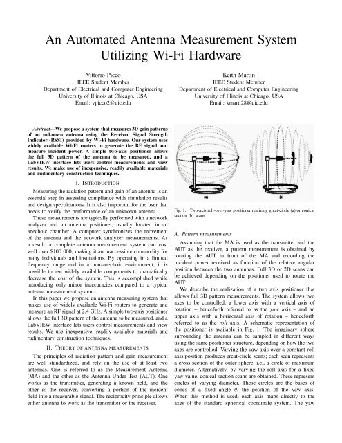
An Automated Antenna Measurement System
Utilizing Wi-Fi Hardware
Vittorio Picco
IEEE Student Member
Department of Electrical and Computer Engineering
University of Illinois at Chicago, USA
Email: vpicco2@uic.edu
Keith Martin
IEEE Student Member
Department of Electrical and Computer Engineering
University of Illinois at Chicago, USA
Email: kmarti28@uic.edu
Abstract—We propose a system that measures 3D gain patterns
of an unknown antenna using the Received Signal Strength
Indicator (RSSI) provided by Wi-Fi hardware. Our system uses
widely available Wi-Fi routers to generate the RF signal and
measure incident power. A simple two-axis positioner allows
the full 3D pattern of the antenna to be measured, and a
LabVIEW interface lets users control measurements and view
results. We make use of inexpensive, readily available materials
and rudimentary construction techniques.
I. INTRODUCTION
Measuring the radiation pattern and gain of an antenna is an
essential step in assessing compliance with simulation results
and design specifications. It is also important for the user that
needs to verify the performance of an unknown antenna.
These measurements are typically performed with a network
analyzer and an antenna positioner, usually located in an
anechoic chamber. A computer synchronizes the movement
of the antenna and the network analyzer measurements. As
a result, a complete antenna measurement system can cost
well over $100 000, making it an inaccessible commodity for
many individuals and institutions. By operating in a limited
frequency range and in a non-anechoic environment, it is
possible to use widely available components to dramatically
decrease the cost of the system. This is accomplished while
introducing only minor inaccuracies compared to a typical
antenna measurement system.
In this paper we propose an antenna measuring system that
makes use of widely available Wi-Fi routers to generate and
measure an RF signal at 2.4 GHz. A simple two-axis positioner
allows the full 3D pattern of the antenna to be measured, and a
LabVIEW interface lets users control measurements and view
results. We use inexpensive, readily available materials and
rudimentary construction techniques.
II. THEORY OF ANTENNA MEASUREMENTS
The principles of radiation pattern and gain measurement
are well standardized, and rely on the use of at least two
antennas. One is referred to as the Measurement Antenna
(MA) and the other as the Antenna Under Test (AUT). One
works as the transmitter, generating a known field, and the
other as the receiver, converting a portion of the incident
field into a measurable signal. The reciprocity principle allows
either antenna to work as the transmitter or the receiver.
Fig. 1. Two-axis roll-over-yaw positioner realizing great-circle (a) or conical
section (b) scans
A. Pattern measurements
Assuming that the MA is used as the transmitter and the
AUT as the receiver, a pattern measurement is obtained by
rotating the AUT in front of the MA and recording the
incident power received as function of the relative angular
position between the two antennas. Full 3D or 2D scans can
be achieved depending on the positioner used to rotate the
AUT.
We describe the realization of a two axis positioner that
allows full 3D pattern measurements. The system allows two
axes to be controlled: a lower axis with a vertical axis of
rotation – henceforth referred to as the yaw axis – and an
upper axis with a horizontal axis of rotation – henceforth
referred to as the roll axis. A schematic representation of
the positioner is available in Fig. 1. The imaginary sphere
surrounding the antenna can be sampled in different ways
using the same positioner structure, depending on how the two
axes are controlled. Varying the yaw axis over a constant roll
axis position produces great-circle scans; each scan represents
a cross-section of the outer sphere, i.e., a circle of maximum
diameter. Alternatively, by varying the roll axis for a fixed
yaw value, conical section scans are obtained. These represent
circles of varying diameter. These circles are the bases of
cones of a fixed angle θ, the position of the yaw axis.
When this method is used, each axis maps directly to the
axes of the standard spherical coordinate system. The yaw

axis is equivalent to movement in the θ direction, and the
roll axis is equivalent to movement in the φ direction. To
avoid cumbersome coordinate conversions, the conical section
method is adopted here.
From this procedure a relative pattern measurement is
obtained. In order to obtain an absolute measurement of an
antenna’s gain, an additional measurement must be performed.
B. Gain measurements
Gain measurements are obtained by first aligning the AUT
and the MA along the maximum found in the pattern measurement.
Then, different techniques can be used to find the
absolute gain of the AUT. Two common methods are the gain
transfer (or gain comparison) method, and the three-antenna
method. An extensive description of these and other techniques
can be found in [1].
The gain transfer method is based on the use of an antenna
of known (standard) gain G sg , whose received power, (P sg ), is
compared to the received power measured by the AUT, (P aut ).
The gain of the antenna under test, (G aut ) is then found as:
G aut = G sg + P aut − P sg , (1)
all quantities expressed in dB.
The three-antenna method is used when no standard gain
antenna is available. In this case three antennas, all of unknown
gain, are used; three measurements are taken, one for each of
three combinations of transmitting and receiving antennas. For
each measurement the Friis transmission equation is used and
the gain of all three antennas can be found by solving a system
of three equations in three unknowns, each one of the form:
(G a ) dB + (G b ) dB = 20 log 10
( 4πR
λ
C. Polarization effects
) ( )
Prb
+ 10 log 10 .
P ta
The MA can be linearly or circularly polarized. If the MA
and AUT are both linearly polarized, the polarization of the
AUT can be found and the co- and cross-polarization patterns
can be measured. By properly mounting the MA and AUT the
user can ensure that only the co- or cross-polarized pattern is
measured in a 2D scan. This is not possible when performing
a 3D scan; therefore, two scans must be performed, rotating
the MA by 90 degrees between each scan.
If one antenna is circularly polarized and the other linearly
polarized, polarization mismatch can no longer occur. However,
no polarization information can be obtained, and the
gain measurement obtained will be 3 dB lower than the actual
value.
All these factors can lead to substantially different designs
and operating procedures. In the following section the details
of our approach are presented and our rationale explained.
A. RF architecture
III. DESCRIPTION OF SYSTEM
1) Approach: The design of the RF section is inspired
by a main competition requirement: a system operating at
(2)
a frequency of 2.4 GHz. Many consumer devices radiate in
this frequency, including Wi-Fi (IEEE 802.11 b/g) and Bluetooth
(IEEE 802.15) devices, cordless phones, and microwave
ovens. This results in significant interference in the 2.4 GHz
band. However, this also makes a multitude of inexpensive
RF devices accessible to the designer. In addition, the Wi-
Fi standard provides mechanisms implemented at both the
physical and data link layers to avoid collisions, reject noise,
and even estimate the power of a received signal. For these
reasons, our design is based on the use of two inexpensive
and widely available Wi-Fi routers. One router acts as a
transmitter, generating an RF signal. The other measures the
received power of this signal, allowing antenna gain and
pattern measurements to be made.
The IEEE 802.11 family of protocols envisions “an optional
parameter that has a value of 0 through RSSI Max. This parameter
is a measure by the PHY of the energy observed at the
antenna [. . . ]. RSSI is intended to be used in a relative manner.
Absolute accuracy of the RSSI reading is not specified” [2].
This generic definition is implemented by manufacturers in
different ways, with the goal of providing the user a visual
estimation of the strength of a Wi-Fi network. The RSSI is
computed by estimating the power in the preamble of a Wi-Fi
beacon. An Access Point (AP) transmits this beacon repeatedly
at fixed intervals, broadcasting basic information about the
Wi-Fi network that the AP is creating. Devices that receive
this beacon generate an estimate of the incident signal power.
This mechanism allows us to obtain not only a received power
estimate, but also to discriminate between different networks,
and obtain a measure with improved noise immunity.
The router chosen to function as both the signal generator
and received power meter is the Linksys WRT54G. This choice
is motivated by two main factors. The first is that according
to the manufacturer’s specifications, Linksys routers provide
their RSSI reading as an integer between 0 to 100. This
appears to be the finest quantization of the RSSI measure
offered by commercial routers, resulting in better sensitivity
to small RSSI changes. The second reason is that the Linksys
WRT54G supports customized firmware maintained by a large
open source community. This open source firmware allows the
user to manipulate otherwise inaccessible parameters, such as
the transmit power and the beacon transmission interval. An
SSH shell interface is also available in some versions, allowing
command line control of the device. We chose the dd-wrt v24
Micro-plus firmware, which specifically allows SSH access.
2) Calibration: RSSI is a precise measure of the incident
power, but not an accurate one. While repeated tests under the
same conditions lead to repeatable results, the result cannot be
used to directly measure incident power. Calibration is needed
to relate RSSI to gain. To calibrate the system, the following
procedure is adopted. Any antennas can be used as the MA
and the AUT; neither needs to be characterized precisely. A
splitter allows the signal received by the AUT to be sent to
the receiving router and to a spectrum analyzer. The router
RSSI and spectrum analyzer measurements are recorded for
a range of transmitter power levels. The transmitted power is

Fig. 2. Incident power on the AUT measured using RSSI and a spectrum
analyzer
Fig. 3. Difference between the RSSI value returned by the router and the
spectrum analyzer measurement as function of the RSSI itself
varied in increments of 3 dB to cover its full dynamic range.
The router RSSI readings and the spectrum analyzer power
measurements are shown in Fig. 2.
The nonlinearities that appear in the spectrum analyzer
measurement are caused by differences between the desired
transmitted power and the actual transmitted power. The RSSI
is linear within an approximately 30 dB range of incident
power.
The difference between the two measurements is shown
in Fig. 3. It can be seen that the difference between the
two readings is small for high levels of received power and
increases when the signal strength decreases. The measured
differences are interpolated using a third order polynomial
estimator, which allows a correction coefficient to be computed
from the following function:
C = −0.00057 ∗ RSSI 3 − 0.0836 ∗ RSSI 2 +
− 4.1314 ∗ RSSI − 61.863. (3)
This correction coefficient is applied to the RSSI values
obtained from the router, allowing the RSSI values to match
the power measurements obtained from the spectrum analyzer.
This calibration operation is advisable, but it is not strictly
necessary. Since the routers proved to behave sufficiently
linearly, the RSSI reading could be used directly as a power
estimate, adding only a few decibels of uncertainty in the
measured result. Because the routers are mass produced, it
may also be possible to assume that all routers of this model
and version number will behave similarly. This would allow
the same calibration to be reused.
3) Pattern measurement: Our LabVIEW interface allows
fully automated measurement of radiation patterns in either
principal plane. The user can specify which principal plane to
scan, the angle to scan, and the angular separation between
data points. The user can also opt to average several measurements
for each data point. The computer uses the router’s
SSH interface to retrieve RSSI measurements and controls the
driver used to rotate the positioner. Once the desired angular
span is covered, the normalized pattern is displayed on a polar
plot.
This procedure is valid regardless of the MA used, given
that care is taken in mounting the antennas so that they
are co-polarized. Nonetheless, to avoid reflections from the
environment it is advisable to choose a directive antenna with
a narrow main lobe. The MA should be in the far field of the
AUT, with its main lobe pointed directly at the AUT.
For a 3D scan two sets of measurements are needed to avoid
spurious cross-polarization effects. The MA is first mounted
to produce a vertically polarized field, and both axes are
scanned. Then the MA is rotated 90 degrees and the scans
are repeated. The first measurement returns the theta-polarized
part of the radiation pattern, while the second returns phipolarized
component. The two components can be combined
together to obtain the total radiation pattern. Because the
received electric field is measured only in terms of power
(i.e. magnitude squared), the two sets of measurements are
summed in this way:
√
G aut = G 2 θ + G2 φ . (4)
4) Gain measurement: To obtain an absolute gain measurement
we use the gain comparison technique. This method
requires a standard gain antenna, but offers some advantages
over the three antenna method. The three-antenna method
requires knowledge of many parameters: the distance between
the antennas, the transmitted power, and an accurate measure
of the received power. In addition, all three antennas must
be identically aligned and impedance matched, and reflections
need to be minimized. Most of these variables cannot be
rigorously controlled in our system. The estimated gain proved
to be unreliable, with large variations between trials.
In the gain comparison method, the only parameters required
are the gain of a known antenna and received power
measurements obtained with the known antenna and the AUT.
This implies that as long as the transmitted power and the
distance between the MA and AUT are not changed, the power
incident on the receiving antenna will be constant. In order to

Fig. 4.
3 GHz dipole antenna
Fig. 5.
2x2 array of microstrip patch antennas
further improve the measurement, multiple RSSI readings are
taken for a range of transmitter power levels and averaged. It is
important to remark that the MA and the standard gain antenna
serve different purposes. The MA works as a transmitter and
does not need to be known, while the standard gain works as
a receiver and needs to have a known absolute gain.
In industry, expensive standard gain horns are normally
used for gain comparison measurements. To minimize the
number of antennas users need to purchase, we determined
the gain of our MA. Users can then use this MA as a standard
gain antenna when performing a gain measurement. Any user
supplied antenna can be used as the MA during the gain
measurement. To determine the gain of our MA, we performed
a gain comparison measurement using a half-wave dipole. The
gain of the dipole can be determined analytically to be 2.1 dBi.
This antenna was available in our lab at no cost, and is only
needed once to determine the gain of the MA.
5) Antenna selection: A planar Yagi antenna is selected
to serve as the MA during pattern measurements, and as the
standard gain during gain measurements. A linearly polarized
antenna was chosen because linearly polarized antennas are
widely available for use in Wi-Fi. The Yagi is a directive
antenna, which helps minimize the effect of reflections. The
gain of the Yagi is determined by performing a gain comparison
measurement with a half-wave dipole, allowing it to also
function as a standard gain. While the dipole offers a known
gain and can be constructed easily, its low directivity would
result in more reflections from the environment. Therefore, a
dipole was not chosen as the MA.
To validate the system, we chose to test a 2x2 planar array
of microstrip patch antennas. This antenna is also linearly
polarized. Its array factor can be computed analytically, and
its far field pattern can be determined through simulation.
Comparing our measurements to the analytical and simulation
results will allow the performance of our system to be judged.
The dipole, patch array, and Yagi antennas are shown in
Fig. 4, 5, and 6 respectively. The coordinate system used to
measure each antenna is also indicated.
Fig. 6.
5-element Yagi antenna
B. Two-axis positioner design and assembly
The positioner is designed with three objectives in mind.
First, it must be able to rotate the AUT with the necessary
precision, and provide a stable and repeatable platform for
measurements. Second, it must cause minimal scattering of
the incident field, so that the behavior of the AUT is not
influenced by the structure. Finally, constructing the positioner
needs to be within the capabilities of students who may not
have extensive experience with fabrication.
We elected to use stepper motors to move the positioner.
Stepper motors allow rotation in predetermined increments,
so they allow the positioner to be rotated through the desired
angle by simply specifying the number of steps to move. The
size of each step is extremely consistent, allowing open loop
control of the motors. We configured the drive to operate
in microsteps, which provides the lowest level of vibration
and highest control of the positioner. In this mode, each
step rotates the shaft of the motor 0.225 ◦ . The motors are
driven by a Xylotex 3-Axis Stepper Motor Driver Board. This
board accepts signals from a PC parallel port, and provides
the necessary outputs for driving stepper motors. The driver,
motors, and power supply are available as a kit from Xylotex,

Fig. 7.
Xylotex stepper motor driver board
Fig. 9.
Column supporting the upper disc and the roll wheel
Fig. 8. Yaw axis motor, belt and pulley. The roll motor is mounted on the
large yaw pulley
simplifying the design.
A stepper motor drives each axis through a belt and pulley
system. While a direct drive between a wheel on the shaft of
the motor and the base of the column was initially considered,
this was abandoned when it was found that this would require
the base to be perfectly concentric. The belt drive allows
consistent, repeatable movements even if the base is not
completely circular. In the yaw axis the motors operate at a
gear ratio of approximately 17:1. This equates to a single step
precision of 0.013 ◦ . To maximize accuracy, the exact gear ratio
is determined empirically after the system is constructed.
The roll axis is driven by a stepper motor attached to the
base of the column. This reduces the effects of scattering from
the conductive body of the motor. Here the belt drive also
allows increased separation between the motor and the axis.
The gear ratio is approximately 6:1, resulting in a single step
rotation of 0.038 ◦ .
The column is constructed of 1.25 in (3.18 cm) oak dowels,
with the ends attached to wooden disks using mortise and
tenon joints. The disks are fabricated to make this joint strong
and easy to assemble. Each disk is made by laminating several
0.125 in (0.32 cm) thick disks together. A set of three disks
is laminated together, and 1.25 in (3.18 cm) holes are drilled
into the disks to accept the dowels. The holes are located
120 ◦ apart using a geometric construction. Two more disks
are then laminated onto the drilled disk, so that the finished
disk has three holes that are guaranteed to be of equal depth.
This process is repeated for a second disk. The dowels are
then glued into each hole in the disks, resulting in a strong
and square column.
The largest available 0.125 in (0.32 cm) thick disks were 10
in (25.4 cm) in diameter, which did not provide enough room
to mount the roll axis motor. Therefore, the entire column was
then attached to the next largest available disk, an 18 in (45.7
cm) diameter, and 1 in (2.54 cm) thick circle. This disk came
with a rounded edge. To make the edge more suitable for a
belt drive, the radius was removed using a band saw at the
UIC machine shop. The work was performed at no cost. The
disk was mounted on a 12 in (30.5 cm) diameter turntable
bearing, which was then fixed to a 24 in x 24 in (61 cm x 61
cm), 0.75 in (1.90 cm) thick plywood base.
The centers of the 18 in (45.7 cm) disk and the disk
at the bottom of the column were found using geometric
construction. A hole was drilled in the disk at the bottom
of the column, so that the center of the 18 in (45.7 cm) disk
would be visible when the column was centered on the larger
disk. The column was then secured to the base using wood
screws.

Fig. 10. Roll axis complete with roll pulley, shaft, bearings and belt flange.
The shaft is cut longitudinally to allow for easy AUT connection with, for
example, double-sided tape, like shown in this figure
To allow rotation in the roll direction, an additional bearing
was needed. The bearing is supported by a section of 2 in
x 4 in (5.08 cm x 10.16 cm) lumber attached to the top of
the column. A 1.25 in (3.18 cm) diameter hole is drilled in
this bearing block to accept a bearing and a shaft to mount
the antenna. The hole is located high enough to allow the
antenna to roll through 360 ◦ , and is offset from the center of
the column so that the antenna can be mounted on the yaw
axis of rotation. To prevent scattering from a metallic bearing,
a plastic sleeve bearing is selected. This bearing fits into the
bearing block and is held in place by a flange. The bearing
accepts a 1 in (2.54 cm) oak dowel, allowing the shaft to turn
freely while being held orthogonal to the yaw axis. A pulley
is fabricated from 6 in (15.24 cm) diameter, 0.125 in (0.32
cm) thick disks, and secured to the dowel using a plastic shaft
collar. A plastic shaft collar with mounting holes on its face
was not available, so holes are drilled through the collar and
the pulley so that nylon machine screws can be used to attach
the pulley to the shaft.
Obtaining pre-made belts in the correct sizes also proved
difficult, so we chose to fabricate our own belts. The belts are
constructed out of several layers of adhesive tape. To construct
the belts, the required circumference is measured. Then the
pulleys are clamped to a table to provide a stable surface. The
distance between the pulleys determines the circumference of
the belt. To provide durability and a high friction interface
between the belt and pulleys, the inner surface of the belt is
made of duct tape. Several layers of Scotch brand transparent
tape are then applied over the duct tape, followed by a final
outer layer of duct tape. This method produces an inexpensive
and resilient belt in any length desired.
The roll axis motor must rotate with the column when it
is moved around the yaw axis, so it is mounted to the base
of the column. We fabricated our own mount from a 0.125 in
(0.32 cm) thick 1 in x 1 in (2.54 cm x 2.54 cm) angle iron
profile. First, we cut two 3.5 in (8.89 cm) long segments from
the profile. Using a #5 (0.522 cm) drill bit, we then drilled
holes in each segment to match the mounting holes on the
face of the motor. On the other side of the profile, we drilled
and countersunk holes for wood screws. The two profiles are
attached to the motors using long #10 (0.483 cm) machine
screws and nuts, which are then cut to length. Nylon spacers
are placed underneath the mount so that the height of the motor
can be adjusted if necessary. This allows the tension in the belt
to be altered. Wood screws secure the motor to the base of the
column. To enhance friction between the motor and the belt,
a 1 in (2.54 cm) soft rubber wheel is used as the drive pulley
for the motor.
The yaw axis motor is suspended upside down to allow its
shaft to be in the same plane as the base of the column. A
brace is constructed of 2 in x 4 in (5.08 cm x 10.16 cm)
lumber, held together by wood screws. Slots are cut in the top
of the brace so that the position of the motor can be adjusted
if necessary, as when installing or removing the belt. Long
#10 (0.483 cm) machine screws between the mounting holes
of the motor and the slots in the brace secure the motor. A 1
in (2.54 cm) soft rubber drive wheel is used as a pulley here
as well. The brace is secured to the plywood base plate using
right angle joist brackets.
In addition to the positioner, we also needed to hold the
MA in a fixed position. The base of the MA mount is an
18 in x 18 in (45.72 cm x 45.72 cm) square cut from a 3/4
in (1.90 cm) thick sheet of plywood. Self-adhesive felt feet
are placed under the base to improve its stability. A 36 in
(91.44 cm) long segment of 2 in x 4 in (5.08 cm x 10.16
cm) lumber is oriented vertically above the center of the base.
Right angle joist brackets are used to ensure that the vertical
segment is normal to the base, and wood screws are used
to secure it to the base. The mount is tall enough so that
the height of the MA can be adjusted so that it is aligned
with the AUT. The mount is suitable for attaching several
antenna geometries. The mounting procedure is similar to that
used with the AUT. Styrofoam blocks are placed between the
mount and the antenna to prevent anomalies caused by locating
microstrip lines next to dielectric materials other than air. The
antenna is secured using double-sided tape. Other antennas,
such as the dipole, can be secured using nylon cable ties.
C. Software
A LabVIEW application is developed to control the movement
of the positioner and to retrieve the RSSI measurements
from the router. LabVIEW makes it easy to develop a sophisticated
GUI and a hardware interface suitable for motor
control.
The positioner’s motions are controlled using the computer’s
parallel port. The mapping of the data register of the parallel
port is shown in Table I.
The LabVIEW program determines the direction and
amount of rotation, and computes the number of micro-steps
necessary. It then applies the appropriate values to the parallel
port. The direction of rotation is controlled by the direction
bit, and the motor rotates one microstep each time a rising
edge occurs on the step bit. The same procedure is valid for
both axes.

TABLE I
PARALLEL PORT DATA REGISTER BITS
Bit # Function
0 Direction axis 1
1 Stepping axis 1
2 Direction axis 1
3 Stepping axis 2
The program Plink is used to communicate with the router.
Plink is a freeware tool that provides a Windows-compatible
SSH client. Combined with the dd-wrt firmware, it allows an
SSH connection to be established automatically. LabVIEW executes
Plink, opens an SSH connection and authenticates itself
as root user, executes the command wl -rssi, and reads
the standard output of Plink to retrieve the RSSI measure.
The procedure is completely automated and requires no user
intervention.
The program allows the user to rotate the axes and take
measurements manually, or to run automated scans of the
principal planes. To perform an automated scan, LabVIEW
executes a series of movements, each followed by an RSSI
measure. The span, angular step size and axis to control
are defined by the user, as is the number of RSSI samples
to collect and average for each position. The program uses
the interpolator polynomial described in the RF architecture
section to automatically determine the correction to be applied.
When the scan is completed the data collected are saved as
an ASCII text file and presented to the user in the form of a
polar plot. During the scan operation no user intervention is
required at all.
The speed of a scan is determined by the amount of movement
requested, by the step size, and by the number of samples
to average. A 360-degree scan with steps of 5 degrees and 8
RSSI samples per position takes approximately 20 minutes.
By combining multiple scans for different AUT positions in
an environment such as MATLAB, full 3D patterns can be
obtained from the raw ASCII text files saved by LabVIEW.
For the purpose of demonstrating the operation and capabilities
of the system, only 2D cuts are presented in the Test Results
section.
IV. BILL OF MATERIALS
Description Source Cost ($)
RF Measurement
Linksys WRT54G, 2x Amazon 113.08
Ethernet cable, 10 ft Amazon 3.95
PCB Patch Antenna Amazon 34.95
PCB Yagi Antenna Amazon 32.95
RP-TNC / N-m, 2x Amazon 9.96
Adpt N-f / SMA, 2x Amazon 8.26
Adpt SMA-f / SMA-f, 2x Digikey 8.90
SMA cables, 4 ft, 2x L-com.com 36.00
Software
LabVIEW student license NI.com 59.95
Positioner control
Motor kit xylotex.com 310.00
DB25 10 ft extension Amazon 3.99
Braided wire Home Depot 5.00
Positioner hardware
Plywood base Home Depot 7.00
18 in Wood Circle Lowes 13.17
12 pk 10 in Wood Circle craftparts.com 11.88
6 in Wood Circle, 12x craftparts.com 7.44
1 1/4 in x 36 in Dowel, 3x craftparts.com 18.75
12 in Turntable McMaster 10.67
8 ft 2 in x 4 in Lumber Home Depot 1.98
1in x 36in Oak Dowel Home Depot 4.37
Acetal Flanged Bearing McMaster 9.60
Slimline Drive Roller, 2x McMaster 59.36
Transparent Tape, 1/2 in Staples 7.49
Duct Tape, black Staples 7.99
1 in x 1 in Angle Iron Home Depot 7.10
Clamp on Shaft Collar McMaster 14.39
Nylon Screws 2in McMaster 7.23
Nylon Hex Nuts, 3/8in McMaster 6.24
Plastic Mesh Flange Joann fabric 0.60
Tension Pins, Spacers Home Depot 15.16
Machine Screws and Nuts McMaster 27.05
Screws, Joist Angles, Glue Menard’s 16.01
Carpet Tape Ace Hardware 4.92
12 3/4in Felt Pads Home Depot 3.61
Shipping costs, total 35.46
TOTAL 924.46
V. TEST RESULTS
The performance of the system was evaluated by measuring
the far field patterns of the patch array, dipole, and Yagi antennas.
The test was performed outdoors to minimize the effect
of reflections, in the area behind a team member’s home. The
test setup is shown in Fig. 11. The test area was approximately
5 m x 5 m square, with the main lobe of the MA pointed at a
wooden fence. The positioner and MA were placed on tables
to elevate them above the ground. The ground consisted of a
grass lawn and a concrete surface. The positioner was placed
over the grass region, as we felt this would minimize the effect
of scattering on the measurement. The relative permittivity of
soil, ɛ r , is approximately 3, compared to 4.5 for concrete. As
will be shown below, the ground was the largest source of
reflections. A 360 ◦ scan in 5 ◦ increments was made in both
principal planes of each antenna. Eight samples were averaged
in each position.
To validate the test results, the far fields of the patch array,
Yagi and dipole antenna were simulated using FEKO. The
curved microstrip feed structure of the patch array proved
difficult to replicate in FEKO. Therefore, we simulated each
patch with its own feed, with all the patches feed in phase and
with the same amplitude. The patch is also simulated with an
infinite substrate. This provides a reasonable approximation of
the far field pattern of the patch array. The measured values

Fig. 11.
Outdoor measurement setup
Fig. 13.
Dipole antenna, φ principal plane
defined pattern of the half-wave dipole, we can conclude that
our system provides reliable pattern measurements.
Fig. 12.
Dipole antenna, θ principal plane
are normalized, and superimposed with the simulation results
to facilitate comparison.
A. Half-wave dipole
The pattern of the dipole is well known and can be
determined analytically with relative ease. Because of this,
measuring a dipole will provide an excellent example of the
performance of our system. In the θ plane, the half-wave dipole
is expected to have a toroidal pattern. Our measured results
clearly show this toroidal pattern, with nulls at 90 ◦ and 270 ◦ .
Both the simulated pattern and the measured pattern are shown
in Fig. 12. While some irregularities are present, the distinct
pattern of the dipole is readily apparent.
In the φ plane, the half-wave dipole is expected to have a
perfectly circular pattern. The measured result and simulation
results are shown in Fig. 13. Some irregularities between
measured and simulated data are expected, and the measured
results do not show an extreme deviation from the expected
circular pattern. By comparing our test results to the well
B. 2x2 patch array
Based on the simulation results, the patch array is expected
to produce a single, large lobe. This is confirmed by an
analytical computation of the array factor of a 2 by 2 planar
array. Because the simulation is performed with an infinite
substrate, the actual results will show some variation due
to diffraction effects from the finite substrate. The measured
results in the θ plane are shown in Fig. 14 along with the
simulation results. The measured results clearly show a single
large lobe, with a small back lobe. Small side lobes are also
present; these may be the results of the finite substrate of the
array. Due to the symmetry and recurrence of these features in
multiple measurements, we do not believe they are spurious.
They are also visible in the φ plane, as seen in Fig. 15.
The large main lobe in the φ plane coincides well with the
simulation results, and the small side lobes are present here
as well, further proof that they are legitimate.
While conducting the measurements of the patch array, we
were able to observe the effect of reflections off the ground.
These were first recognized as distinctive asymmetrical lobes
in the θ plane pattern of the array. These lobes occurred when
the broadside lobe and the backlobe were pointed towards the
ground. Comparing Fig. 16 (left) with Fig. 14, the large lobes
at 300 ◦ and 145 ◦ are very noticeable.
To confirm that this effect was due to reflections off the
ground, the scan was repeated while rotating the positioner
in the opposite direction. Because the 0 ◦ position is always
assigned to the start of the scan, with the angle increasing as
the scan progresses, the pattern should be reflected by 180 ◦ .
This is indeed the case, as is shown by Fig. 16 (right). In this
case the main lobe is pointed at the ground at 60 ◦ , and the
back lobe is pointed at the ground at 225 ◦ . Fig. 16 (right) is
a near perfect reflection of Fig. 16 (left).

Fig. 14.
Patch array antenna, θ principal plane
Fig. 17.
Yagi antenna, θ principal plane
Fig. 15.
Patch array antenna, φ principal plane
Fig. 16. Patch array antenna, θ principal plane scanned clockwise (left) and
counter-clockwise (right) showing reflection of side lobe positions
The surface of the ground was wet from recent rain, which
likely increased the relative permittivity of the surface and
increased its reflection coefficient. To eliminate this effect, we
performed the scan again, this time scanning with the yaw axis
of the positioner. To maintain the co-polarization with the MA,
both the AUT and the MA were rotated. In this configuration,
the AUT is never pointed at the ground. Fig. 14 shows that the
ground reflections are no longer present when this method is
used. Unless otherwise indicated, all results shown here were
gathered using yaw scans. This effect may be diminished when
the surface is dry, however, this test condition was difficult to
obtain at our locale.
C. 5-element Yagi
Unlike the dipole and the patch array, an analytical computation
cannot be made to confirm the simulation results of the
Yagi antenna. However, our previous measurements have been
very representative of the results obtained analytically and
through simulation. We show that the measured pattern of the
Yagi antenna also represents the expected pattern accurately.
The entire Yagi antenna is simulated, including the feed
structure, on a finite dielectric substrate. In the θ principal
plane, a large main lobe is expected, along with a smaller
back lobe. The measured results in Fig. 17 show a large main
lobe that coincides very well with the simulation results. A
small additional back lobe is present. This may be the result
of scattering caused by the coaxial feed cable mounted on the
back of the antenna.
D. Gain
The gain measurement procedure is tested on the 5-element
Yagi, which is advertised as having an 8.5 dBi gain, and on
the patch array, which is advertised as having an 11.5 dBi
gain. A half-wave dipole available in the lab is used as the
standard gain antenna. A half-wave dipole is expected have a
gain of 2.15 dBi. However, the dipole at hand was designed to
operate at 3 GHz, making it slightly smaller than a half-wave
length at 2.4 GHz. Therefore, we estimate the gain at 2.4 GHz
to be 2 dBi. Once the gain of the Yagi antenna is known, the
half-wave dipole is not needed. The Yagi itself can be used as
the standard gain antenna for future gain measurements. When
performing a gain measurement any antenna can be used as

TABLE II
GAIN MEASUREMENT TEST, YAGI ANTENNA
P t [mW] G sg [dBi] P sg [dBm] P aut [dBm] G aut [dBi]
128 2 -41.0 -35.0 8.0
64 2 -44.9 -38.9 8.0
32 2 -49.0 -39.9 11.1
16 2 -50.5 -41.4 11.1
8 2 -53.6 -44.9 10.7
Average 9.8
TABLE III
GAIN MEASUREMENT TEST, PATCH ARRAY
P t [mW] G sg [dBi] P sg [dBm] P aut [dBm] G aut [dBi]
128 2 -43.6 -37.6 7.9
64 2 -49.1 -39.1 12.0
32 2 -51.5 -41.9 11.6
16 2 -53.9 -44.3 11.6
8 2 -56.3 -48.3 10.0
Average 10.6
the MA. When measuring the gain of the Yagi in our tests
the patch array was used as the MA. The Yagi was used as
the MA when measuring the gain of the patch array. The gain
measurements of the Yagi are available in Table II.
The gain measurements of the patch array are presented in
Table III. The Yagi antenna shows a larger discrepancy from
its nominal value (1.3 dBi difference) than the patch array
(0.9 dBi difference). It is not known how the manufacturer
determines the gain of these antennas, or what tolerance is
expected in the nominal gain. Additional errors may be introduced
by mechanical misalignment of the antennas, imperfect
impedance matching, and by operating in a non-anechoic environment.
In particular, the Yagi antenna’s reflection coefficient
S 11 proved to be very susceptible to perturbations in its near
field. Even placing styrofoam in contact with the antenna’s
microstrip had a significant effect on the return loss. These
near field effects may have contributed to the discrepancy in
the gain measurement. However, as the manufacturer provides
only the nominal gain, more information would be needed to
adequately judge our gain measurements.
For these reasons, we believe that the goal of ±0.5 dB
error in the gain measure can be achieved in an anechoic
environment, provided that particular care is taken to attach
the antennas to the positioner without influencing the reactive
near field of the antenna.
VI. CONCLUSION
We have shown that it is possible to realize a complete
antenna measurement system operating at 2.4 GHz using only
inexpensive and readily available equipment. The designed
system is able to measure accurate radiation patterns even
in non-anechoic environments. Precaution should be taken in
choosing the axes of rotation so as to avoid obvious reflections
from surfaces such as the floor or walls, depending on the
operating environment. Radiation patterns in each principal
plane can be measured automatically. In principle both 2D
and 3D radiation patterns can be measured, although the time
required for a complete 4π srad scan may be large.
The gain measure proved to be more difficult because of the
large number of variables involved that need to be controlled.
By minimizing user errors such as polarization mismatch, a
reasonable argument is presented that the system could achieve
± 0.5 dB gain accuracy in an anechoic environment.
ACKNOWLEDGMENT
The authors would like to thank Prof. Konrad Kaczmarski of
UIC for his numerous design suggestions, Tadahiro Negishi of
UIC for the invaluable help in simulating antennas with FEKO,
and Prof. Danilo Erricolo of UIC for his guidance throughout
the project.
REFERENCES
[1] IEEE Standard Test Procedures for Antennas, IEEE Std 149-1979,
Published by IEEE, Inc., 1979
[2] IEEE Standard for Information technology. Local and metropolitan area
networks - Specific requirements. Part 11: Wireless LAN Medium Access
control and Physical Layer Specifications, section 14.2.3.2, IEEE Std
802.11-2007, 2007
[3] C. A. Balanis, Antenna Theory Analysis and Design, 3rd ed., Wiley-
Interscience, 2005
[4] R. H. Bishop, LabVIEW 8 Student Edition, 1st ed., Pearson Education,
2007
[5] K. J. Kaczmarski, An “exact” inverse source reconstruction, Ph.D.
dissertation, University of Illinois at Chicago, Chicago, IL, 2008
Vittorio Picco (S ’09) was born in Mondovì (Cuneo),
Italy, in 1985. He received the B.Sc. in electronic
engineering and the M.Sc. (summa cum laude)
in telecommunications engineering from the Politecnico
di Torino, Italy, in 2007 and 2010, respectively.
He received the M.Sc. in electrical and computer engineering
from the University of Illinois at Chicago
(UIC) in 2010.
Since January 2010 he is pursuing his Ph.D.
degree in electrical and computer engineering at
UIC, in the Andrew Electromagnetics Laboratory.
His research interests include electromagnetic propagation and scattering with
applications to narrowband non-destructive underground imaging, and antenna
design.
Mr. Picco is a member of Eta Kappa Nu.
Keith Martin (S ’11) was born in St. Charles, Illinois,
in 1985. He received the B.S. in electrical engineering
from Northwestern University, Evanston,
Illinois, in 2007.
He has worked as an Electronic Engineer at PEC
Products and a Systems Integration and Technology
Analyst at Accenture. Since August 2011 he is
pursuing his M.S degree in electrical and computer
engineering at UIC, in the Andrew Electromagnetics
Laboratory. His research interests include guided and
free space electromagnetic propagation and the use
of computational methods.
Mr. Martin is a member of Eta Kappa Nu.