( ) Robustness of Local Binary Patterns in Brain MR Image Analysis*

More documents

Recommendations

Info

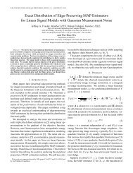
symmetric neighborhood which requires interpolation of intensity values for exact computation. In order to keep computation simple, in this study we decided to use the three rectangular neighborhoods as shown in Fig. 2. g c LBP 8,1 g c LBP A. Rotation Invariant Patterns The LBP P , operator can produce 2 P different output values R from the P neighbor pixels. As g is always assigned to be 0 the gray value of neighbor to the right of g , rotation will result in a different LBP P , value for the same binary R pattern. One way to eliminate the effect of rotation is to perform a bitwise shift operation on the binary pattern P-1 times and assign the LBP value that is the smallest, which is ri now referred to as LBP , (Fig. 3). P R B. “Uniform” Patterns 16,2 A binary pattern is called “uniform” if it contains at most 2 spatial transitions (bitwise 0/1 changes) [1]. Based on this riu2 uniformity concept, a new LBP value ( LBP ) can be c P, R computed by summing the bit values of a rotation invariant binary pattern if it is uniform, or a miscellaneous label P+1 g c LBP 24,3 Fig. 2. The rectangular neighborhoods of LBP used in this study. Gray-shaded rectangles refer to the pixels belonging to the corresponding neighborhood. 00011110 2 = 30 00111100 2 = 60 01111000 2 =120 11110000 2 =240 11100001 2 =225 11000011 2 =195 10000111 2 =135 00001111 2 = 15 LBP ri 8 ,1 = Fig. 3. Example of computing rotation invariant LBP. LBP 1 ri spatial 8 , transitions 15 LBP 00000000 2 0 0 11111111 2 0 8 00000001 2 2 1 00000011 2 2 2 00001011 2 4 9 riu 2 8,1 Fig. 4. Example of computing rotation invariant and uniform LBP. can be assigned if it is nonuniform (Fig. 4). In this study, robustness of simple ( LBP P , ), rotation R ri invariant ( LBP P , ), and rotation invariant and uniform R riu2 ( LBP P, R ) LBP features at three different rectangular neighborhoods (Fig. 2) are tested relative to bias field and rotation. III. APPLICATIONS OF LBP TO MR BRAIN IMAGE ANALYSIS In MRI patient is subjected to different magnetic fields at specific orientations. The protons (hydrogen atoms) in the patient’s body respond to these fields by differential decay and recovery signals, which are acquired by the MR machine and then converted to high contrast images. Due to factors like poor radio-frequency gradient uniformity, static field inhomogeneity, radio-frequency penetration, gradient-driven eddy currents, and patient anatomy and position, pixel intensities in MR images smoothly vary. This variation, known as intensity inhomogeneity/nonuniformity or bias field, has little impact on visual diagnosis, but its impact on the performance of automatic segmentation methods can be catastrophic due to increased overlaps between intensities of different tissues. Furthermore, acquisition times of MRI are generally in the order of 10-20 minutes, during which patients (especially those with Parkinson’s disease) tend to move that results in spatially misaligned images. A common solution for this problem is registration, which may not be favored in some applications due to its computational expense and complexity. Hence, textural descriptors for MR images that are consistent in varying intensities as well as geometric transformations like rotation will be very valuable. A. Experimental Data IV. RESULTS The database used in this study consists of dual (T2 and Proton Density) MR scans from 549 subjects, which are acquired on a Philips Intera 1.5T whole body scanner at Leiden University Medical Center. We used dual-spin echo weighted images (TR/TE1/TE2: 3000/27/120 ms, FLIP: 90) with 220mm FOV, 3mm slice thickness, no slice gap and 256x256 matrix. In order to test robustness of LBP with respect to intensity variations, three simulated bias fields from the BrainWeb MR simulator [10] are used (Fig. 5). These bias fields provide smooth variations of intensity across the image. Furthermore, we applied linear transformation to obtain a new bias field of each with 10%, 20%, 30% and 40% A B C Fig. 5. Examples of simulated bias fields used in this study, where intensity variations are exaggerated for visual purposes.
intensity variations. Based on the conventional assumption that the bias field in MR images is multiplicative [7]-[9], we degraded the original images by multiplying them with the resulting bias fields. B. Evaluation Method The degree of dissimilarity between the LBP values of the original and the degraded (by the bias field and rotation) images is computed on the corresponding normalized LBP histograms using the Bhattacharyya distance (3) and the histogram intersection (4): L ∑ − 1 i= 0 L 1 ( i) ⋅ q( i) d = 1− p (3) B [ p( i) , q( i) ] − ∑ − d = 1 min (4) I i= 0 where p and q are the two histograms with L-bins. The dissimilarity scores for both measures fall in the range of [0,1], where 0 means that the two images are perfectly similar. Please note that as we observed similar results with both measures for all the tests, the following sections provide the results based on only Bhattacharyya measure. C. Robustness to Bias Field We first tested the consistency of LBP relative to the bias field, where several LBP operators are applied on the original images as well as on those degraded by the bias fields. Table I displays dissimilarity scores of this test for all the bias fields and several LBP features, while Fig.6 shows the result of LBP . We observe a steady increase in 8, 1 dissimilarity values with the bias field strength. Bias field B provides the highest dissimilarity score for all strengths, TABLE I EFFECT OF BIAS FIELD ON VARIOUS LBP FEATURES because it has larger spatial variation. All the dissimilarity values are below 0.04%, which shows that the LBP features are robust to the bias fields. D. Robustness to Rotation In order to test the robustness of LBP features relative to rotation, we have rotated the original images by 15°, 30°, 45°, and 60° at clockwise and counterclockwise directions using three different interpolation methods: nearest neighbor, bilinear, and bicubic (presented from the simplest to the most complex, respectively). Fig. 7 displays examples of some of the rotated images. Fig. 7. Examples of T2 (1 st and 3 rd from the left) and Proton Density (2 nd and 4 th from the left) images rotated by 15°, 30°, 45° and 60°, respectively using bicubic interpolation. Table II displays the average dissimilarity scores of this test for all the LBP features when the images are rotated by various angles in both clockwise and counterclockwise directions using three interpolation methods. We generally observe that dissimilarity values decrease when 1) the complexity of the interpolation method increases, 2) the rotation invariancy and the uniformity is introduced to LBP, and 3) the radius of the LBP operator is increased. The former observation is coherent with the fact that the complexity of the interpolation method is directly related to the quality of the resulting rotated image. The second observation is understandable when we consider that the rotation invariant and “uniform” LBP patterns correspond to the primitive microfeatures in the image [1]. Finally, the third observation is meaningful in the sense that as the neighborhood gets bigger, the effect of degradation caused by rotation gets weaker due to the increased radius as well as TABLE II EFFECT OF ROTATION ON VARIOUS LBP FEATURES Values in the table are the dissimilarity scores (10 -4 ). Fig. 6. Robustness of LBP 8,1 relative to varying bias field strength. Values in the table are the dissimilarity scores (10 -2 ).
Page 1: Robustness of Local Binary Patterns

( ) Robustness of Local Binary Patterns in Brain MR Image Analysis*

You also want an ePaper? Increase the reach of your titles

Delete template?

Save as template?