Hypothesis Testing Using z- and t-tests In hypothesis testing, one ...

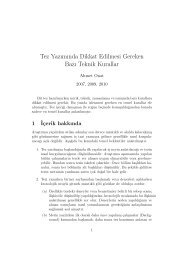
B. Weaver (24-Aug-2010) z- and t-tests ... 1Hypothesis Testing Using z- and t-testsIn hypothesis testing, one attempts to answer the following question: If the null hypothesis isassumed to be true, what is the probability of obtaining the observed result, or any more extremeresult that is favourable to the alternative hypothesis? 1 In order to tackle this question, at least inthe context of z- and t-tests, one must first understand two important concepts: 1) samplingdistributions of statistics, and 2) the central limit theorem.Sampling DistributionsImagine drawing (with replacement) all possible samples of size n from a population, and foreach sample, calculating a statistic--e.g., the sample mean. The frequency distribution of thosesample means would be the sampling distribution of the mean (for samples of size n drawn fromthat particular population).Normally, one thinks of sampling from relatively large populations. But the concept of asampling distribution can be illustrated with a small population. Suppose, for example, that ourpopulation consisted of the following 5 scores: 2, 3, 4, 5, and 6. The population mean = 4, andthe population standard deviation (dividing by N) = 1.414.If we drew (with replacement) all possible samples of 2 from this population, we would end upwith the 25 samples shown in Table 1.Table 1: All possible samples of n=2 from a population of 5 scores.First Second Sample First Second SampleSample # Score Score Mean Sample # Score Score Mean1 2 2 2 14 4 5 4.52 2 3 2.5 15 4 6 53 2 4 3 16 5 2 3.54 2 5 3.5 17 5 3 45 2 6 4 18 5 4 4.56 3 2 2.5 19 5 5 57 3 3 3 20 5 6 5.58 3 4 3.5 21 6 2 49 3 5 4 22 6 3 4.510 3 6 4.5 23 6 4 511 4 2 3 24 6 5 5.512 4 3 3.5 25 6 6 613 4 4 4Mean of the sample means = 4.000SD of the sample means = 1.000(SD calculated with division by N)1 That probability is called a p-value. It is a really a conditional probability--it is conditional on the null hypothesisbeing true.

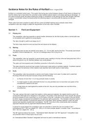
B. Weaver (24-Aug-2010) z- and t-tests ... 2The 25 sample means from Table 1 are plotted below in Figure 1 (a histogram). This distributionof sample means is called the sampling distribution of the mean for samples of n=2 from thepopulation of interest (i.e., our population of 5 scores).6Distribution of Sample Means*54321Std. Dev = 1.02Mean = 4.0002.002.503.003.504.004.505.005.506.00N = 25.00MEANS* or "Sampling Distribution of the Mean"Figure 1: Sampling distribution of the mean for samples of n=2 from a population of N=5.I suspect the first thing you noticed about this figure is peaked in the middle, and symmetricalabout the mean. This is an important characteristic of sampling distributions, and we will returnto it in a moment.You may have also noticed that the standard deviation reported in the figure legend is 1.02,whereas I reported SD = 1.000 in Table 1. Why the discrepancy? Because I used the populationSD formula (with division by N) to compute SD = 1.000 in Table 1, but SPSS used the sampleSD formula (with division by n-1) when computing the SD it plotted alongside the histogram.The population SD is the correct one to use in this case, because I have the entire population of25 samples in hand.The Central Limit Theorem (CLT)If I were a mathematical statistician, I would now proceed to work through derivations, provingthe following statements:

B. Weaver (24-Aug-2010) z- and t-tests ... 31. The mean of the sampling distribution of the mean = the population mean2. The SD of the sampling distribution of the mean = the standard error (SE) of the mean = thepopulation standard deviation divided by the square root of the sample sizePutting these statements into symbols:µ = µ { mean of the sample means = the population mean } (1.1)XXσXσ = { SE of mean = population SD over square root of n } (1.2)XnBut alas, I am not a mathematical statistician. Therefore, I will content myself with telling youthat these statements are true (those of you who do not trust me, or are simply curious, mayconsult a mathematical stats textbook), and pointing to the example we started this chapter with.For that population of 5 scores, µ = 4 and σ = 1.414. As shown in Table 1, µ = µ = 4, andσ = 1.000 . According to equation (1.2), if we divide the population SD by the square root ofXthe sample size, we should obtain the standard error of the mean. So let's give it a try:σ 1.414 = = .9998 1(1.3)n 2When I performed the calculation in Excel and did not round off σ to 3 decimals, the solutionworked out to 1 exactly. In the Excel worksheet that demonstrates this, you may also change thevalues of the 5 population scores, and should observe that σ = σ n for any set of 5 scores youXchoose. Of course, these demonstrations do not prove the CLT (see the aforementioned mathstatsbooks if you want proof), but they should reassure you that it does indeed work.What the CLT tells us about the shape of the sampling distributionThe central limit theorem also provides us with some very helpful information about the shape ofthe sampling distribution of the mean. Specifically, it tells us the conditions under which thesampling distribution of the mean is normally distributed, or at least approximately normal,where approximately means close enough to treat as normal for practical purposes.The shape of the sampling distribution depends on two factors: the shape of the population fromwhich you sampled, and sample size. The following statements illustrate how these factorsinteract in determining the shape of the sampling distribution:1. If the population from which you sampled is itself normally distributed, then the samplingdistribution of the mean will be normal, regardless of sample size. (Even for sample size =1, the sampling distribution of the mean will be normal, because it will be an exact copy ofthe population distribution).X

B. Weaver (24-Aug-2010) z- and t-tests ... 42. If the population distribution is reasonably symmetrical (i.e., not too skewed, reasonablynormal looking), then the sampling distribution of the mean will be approximately normal forsamples of 30 or greater.3. If the population shape is as far from normal as possible, the sampling distribution of themean will still be approximately normal for sample sizes of 300 or greater.So, the general principle is that the more the population shape departs from normal, the greaterthe sample size must be to ensure that the sampling distribution of the mean is approximatelynormal.For many of the distributions that we work with in areas like Psychology and biomedicalresearch, sample sizes of 20 to 30 or greater are often adequate to ensure that the samplingdistribution of the mean is approximately normal (but some more conservative textbook authorsmay recommend 50 or greater). Notice that even for the population of 5 scores we started with,the sampling distribution of the mean for samples of n=2 looks very symmetrical (Figure 1).The sampling distribution of the mean and z-scoresWhen you first encountered z-scores, you were undoubtedly using them in the context of a rawscore distribution. In that case, you calculated the z-score corresponding to some value of X asfollows:zX − µX − µX= = (1.4)σ σXAnd, if the distribution of X was normal, or at least approximately normal, you could then takethat z-score, and refer it to a table of the standard normal distribution to figure out the proportionof scores higher than X, or lower than X, etc.Because of what we learned from the central limit theorem, we are now in a position to computea z-score as follows:zX − µ X − µσ σXnX= = (1.5)This is the same formula, but with X in place of X, and σ in place of σXX. And, if the samplingdistribution of X is normal, or at least approximately normal, we may then refer this value of zto the standard normal distribution, just as we did when we were using raw scores. (This iswhere the CLT comes in, because it tells the conditions under which the sampling distribution ofX is approximately normal.)

B. Weaver (24-Aug-2010) z- and t-tests ... 5An example. Here is a (fictitious) newspaper advertisement for a program designed to increaseintelligence of school children 2 :As an expert on IQ, you know that in the general population of children, the mean IQ = 100, andthe population SD = 15 (for the WISC, at least). You also know that IQ is (approximately)normally distributed in the population. Equipped with this information, you can now addressquestions such as:If the n=25 children from Dundas are a random sample from the general population of children,a) What is the probability of getting a sample mean of 108 or higher?b) What is the probability of getting a sample mean of 92 or lower?c) How high would the sample mean have to be for you to say that the probability of getting amean that high (or higher) was 0.05 (or 5%)?d) How low would the sample mean have to be for you to say that the probability of getting amean that low (or lower) was 0.05 (or 5%)?The solutions to these questions are quite straightforward, given everything we have learned sofar in this chapter. If we have sampled from the general population of children, as we areassuming, then the population from which we have sampled is at least approximately normal.Therefore, the sampling distribution of the mean will be normal, regardless of sample size.Therefore, we can compute a z-score, and refer it to the table of the standard normal distribution.So, for part (a) above:X −µ X −µXX108 −100 8z = = = = = 2.667(1.6)σ σX15 3Xn 252 I cannot find the original source for this example, but I believe I got it from Dr. Geoff Norman, McMasterUniversity.

B. Weaver (24-Aug-2010) z- and t-tests ... 6And from a table of the standard normal distribution (or using a computer program, as I did), wecan see that the probability of a z-score greater than or equal to 2.667 = 0.0038. Translating thatback to the original units, we could say that the probability of getting a sample mean of 108 (orgreater) is .0038 (assuming that the 25 children are a random sample from the generalpopulation).For part (b), do the same, but replace 108 with 92:X −µ X −µXX92 −100 −8z = = = = = − 2.667(1.7)σ σX15 3Xn 25Because the standard normal distribution is symmetrical about 0, the probability of a z-scoreequal to or less than -2.667 is the same as the probability of a z-score equal to or greater than2.667. So, the probability of a sample mean less than or equal to 92 is also equal to 0.0038. Hadwe asked for the probability of a sample mean that is either 108 or greater, or 92 or less, theanswer would be 0.0038 + 0.0038 = 0.0076.Part (c) above amounts to the same thing as asking, "What sample mean corresponds to a z-scoreof 1.645?", because we know that pz≥ ( 1.645) = 0.05. We can start out with the usual z-scoreformula, but need to rearrange the terms a bit, because we know that z = 1.645, and are trying todetermine the corresponding value of X .z =X − µσXX{ cross-multiply to get to next line }z σ = X −µ { add µ to both sides }X X Xz σ + µ = X { switch sides }XX(1.8)X( )= zσ + µ = 1.645 15 25 + 100 = 104.935XXSo, had we obtained a sample mean of 105, we could have concluded that the probability of amean that high or higher was .05 (or 5%).For part (d), because of the symmetry of the standard normal distribution about 0, we would usethe same method, but substituting -1.645 for 1.645. This would yield an answer of 100 - 4.935 =95.065. So the probability of a sample mean less than or equal to 95 is also 5%.The single sample z-testIt is now time to translate what we have just been doing into the formal terminology ofhypothesis testing. In hypothesis testing, one has two hypotheses: The null hypothesis, and the

B. Weaver (24-Aug-2010) z- and t-tests ... 7alternative hypothesis. These two hypotheses are mutually exclusive and exhaustive. In otherwords, they cannot share any outcomes in common, but together must account for all possibleoutcomes.In informal terms, the null hypothesis typically states something along the lines of, "there is notreatment effect", or "there is no difference between the groups". 3The alternative hypothesis typically states that there is a treatment effect, or that there is adifference between the groups. Furthermore, an alternative hypothesis may be directional ornon-directional. That is, it may or may not specify the direction of the difference between thegroups.H0and H1are the symbols used to represent the null and alternative hypotheses respectively.(Some books may use Hafor the alternative hypothesis.) Let us consider various pairs of nulland alternative hypotheses for the IQ example we have been considering.Version 1: A directional alternative hypothesisHH01: µ ≤ 100: µ > 100This pair of hypotheses can be summarized as follows. If the alternative hypothesis is true, thesample of 25 children we have drawn is from a population with mean IQ greater than 100. Butif the null hypothesis is true, the sample is from a population with mean IQ equal to or less than100. Thus, we would only be in a position to reject the null hypothesis if the sample mean isgreater than 100 by a sufficient amount. If the sample mean is less than 100, no matter by howmuch, we would not be able to reject H0.How much greater than 100 must the sample mean be for us to be comfortable in rejecting thenull hypothesis? There is no unequivocal answer to that question. But the answer that mostdisciplines use by convention is this: The difference between X and µ must be large enoughthat the probability it occurred by chance (given a true null hypothesis) is 5% or less.The observed sample mean for this example was 108. As we saw earlier, this corresponds to a z-score of 2.667, and pz≥ ( 2.667) = 0.0038 . Therefore, we could reject H0, and we would act asif the sample was drawn from a population in which mean IQ is greater than 100.3 I said it typically states this, because there may be cases where the null hypothesis specifies a difference betweengroups of a certain size rather than no difference between groups. In such a case, obtaining a mean difference ofzero may actually allow you to reject the null hypothesis.

B. Weaver (24-Aug-2010) z- and t-tests ... 8Version 2: Another directional alternative hypothesisHH01: µ ≥ 100: µ < 100This pair of hypotheses would be used if we expected the Dr. Duntz's program to lower IQ, andif we were willing to include an increase in IQ (no matter how large) under the null hypothesis.Given a sample mean of 108, we could stop without calculating z, because the difference is inthe wrong direction. That is, to have any hope of rejecting H0, the observed difference must bein the direction specified by H1.Version 3: A non-directional alternative hypothesisHH01: µ = 100: µ ≠ 100In this case, the null hypothesis states that the 25 children are a random sample from a populationwith mean IQ = 100, and the alternative hypothesis says they are not--but it does not specify thedirection of the difference from 100. In the first directional test, we needed to have X > 100 bya sufficient amount, and in the second directional test, X < 100 by a sufficient amount in orderto reject H0. But in this case, with a non-directional alternative hypothesis, we may reject H0ifX < 100 or if X > 100, provided the difference is large enough.Because differences in either direction can lead to rejection of H0, we must consider both tails ofthe standard normal distribution when calculating the p-value--i.e., the probability of theobserved outcome, or a more extreme outcome favourable to H1. For symmetrical distributionslike the standard normal, this boils down to taking the p-value for a directional (or 1-tailed) test,and doubling it.For this example, the sample mean = 108. This represents a difference of +8 from the populationmean (under a true null hypothesis). Because we are interested in both tails of the distribution,we must figure out the probability of a difference of +8 or greater, or a change of -8 or greater.In other words, p = p( X ≥ 108) + p( X ≤ 92) = .0038 + .0038 = .0076 .Single sample t-test (whenσ is not known)In many real-world cases of hypothesis testing, one does not know the standard deviation of thepopulation. In such cases, it must be estimated using the sample standard deviation. That is, s(calculated with division by n-1) is used to estimate σ . Other than that, the calculations are aswe saw for the z-test for a single sample--but the test statistic is called t, not z.

B. Weaver (24-Aug-2010) z- and t-tests ... 9∑( X − X) 2X − µXsSSXt( df = n−1) = where s = , and s = =Xs nn−1 n−1X(1.9)In equation (1.9), notice the subscript written by the t. It says "df = n-1". The "df" stands fordegrees of freedom. "Degrees of freedom" can be a bit tricky to grasp, but let's see if we canmake it clear.Degrees of FreedomSuppose I tell you that I have a sample of n=4 scores, and that the first three scores are 2, 3, and5. What is the value of the 4 th score? You can't tell me, given only that n = 4. It could beanything. In other words, all of the scores, including the last one, are free to vary: df = n for asample mean.To calculate t, you must first calculate the sample standard deviation. The conceptual formulafor the sample standard deviation is:s =∑( X − X ) 2n −1(1.10)Suppose that the last score in my sample of 4 scores is a 6. That would make the sample meanequal to (2+3+5+6)/4 = 4. As shown in Table 2, the deviation scores for the first 3 scores are -2,-1, and 1.Table 2: Illustration of degrees of freedom for sample standard deviationScoreDeviationfrom MeanMean2 4 -23 4 -15 4 1-- -- x4Using only the information shown in the final column of Table 2, you can deduce that x4, the 4 thdeviation score, is equal to -2. How so? Because by definition, the sum of the deviations aboutthe mean = 0. This is another way of saying that the mean is the exact balancing point of thedistribution. In symbols:( X − X) = 0∑ (1.11)

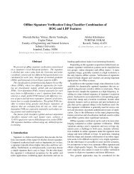
B. Weaver (24-Aug-2010) z- and t-tests ... 10So, once you have n-1 of the ( X − X )deviation scores, the final deviation score is determined.That is, the first n-1 deviation scores are free to vary, but the final one is not. There are n-1degrees of freedom whenever you calculate a sample variance (or standard deviation).The sampling distribution of tTo calculate the p-value for a single sample z-test, we used the standard normal distribution. Fora single sample t-test, we must use a t-distribution with n-1 degrees of freedom. As this implies,there is a whole family of t-distributions, with degrees of freedom ranging from 1 to infinity ( ∞= the symbol for infinity). All t-distributions are symmetrical about 0, like the standard normal.In fact, the t-distribution with df = ∞ is identical to the standard normal distribution.But as shown in Figure 2 below, t-distributions with df < infinity have lower peaks and thickertails than the standard normal distribution. To use the technical term for this, they are leptokurtic.(The normal distribution is said to be mesokurtic.) As a result, the critical values of t are furtherfrom 0 than the corresponding critical values of z. Putting it another way, the absolute value ofcritical t is greater than the absolute value of critical z for all t-distributions with df < ∞ :For df zcritical(1.12).5.4Probability density functionsStandard NormalDistribution.3t-distribution withdf = 10.2.1t-distribution withdf = 20.0-6-4-20246Figure 2: Probability density functions of: the standard normal distribution (the highest peak with thethinnest tails); the t-distribution with df=10 (intermediate peak and tails); and the t-distribution with df=2(the lowest peak and thickest tails). The dotted lines are at -1.96 and +1.96, the critical values of z for atwo-tailed test with alpha = .05. For all t-distributions with df < ∞ , the proportion of area beyond -1.96and +1.96 is greater than .05. The lower the degrees of freedom, the thicker the tails, and the greater theproportion of area beyond -1.96 and +1.96.

B. Weaver (24-Aug-2010) z- and t-tests ... 11Table 3 (see below) shows yet another way to think about the relationship between the standardnormal distribution and various t-distributions. It shows the area in the two tails beyond -1.96and +1.96, the critical values of z with 2-tailed alpha = .05. With df=1, roughly 15% of the areafalls in each tail of the t-distribution. As df gets larger, the tail areas get smaller and smaller,until the t-distribution converges on the standard normal when df = infinity.Table 3: Area beyond critical values of + or -1.96 in various t-distributions.The t-distribution with df = infinity is identical to the standard normal distribution.Degrees of Area beyond Degrees of Area beyondFreedom + or -1.96 Freedom + or -1.961 0.30034 40 0.056992 0.18906 50 0.055583 0.14485 100 0.052784 0.12155 200 0.051385 0.10729 300 0.0509210 0.07844 400 0.0506915 0.06884 500 0.0505520 0.06408 1,000 0.0502725 0.06123 5,000 0.0500530 0.05934 10,000 0.05002Infinity 0.05000Example of single-sample t-test.This example is taken from Understanding Statistics in the Behavioral Sciences (3 rd Ed), byRobert R. Pagano.A researcher believes that in recent years women have been getting taller. She knows that 10 years ago theaverage height of young adult women living in her city was 63 inches. The standard deviation is unknown.She randomly samples eight young adult women currently residing in her city and measures their heights.The following data are obtained: [64, 66, 68, 60, 62, 65, 66, 63.]The null hypothesis is that these 8 women are a random sample from a population in which themean height is 63 inches. The non-directional alternative states that the women are a randomsample from a population in which the mean is not 63 inches.HH01: µ = 63: µ ≠ 63The sample mean is 64.25. Because the population standard deviation is not known, we mustestimate it using the sample standard deviation.

B. Weaver (24-Aug-2010) z- and t-tests ... 12sample SD = s =∑( X − X)n −12 2 2(64 − 64.25) + (66 − 64.25) + ...(63 −64.25)= = 2.549572(1.13)We can now use the sample standard deviation to estimate the standard error of the mean:And finally:s 2.5495Estimated SE of mean = s = = = 0.901(1.14)Xn 8X − µ0 64.25 − 63t = = = 1.387(1.15)s 0.901XThis value of t can be referred to a t-distribution with df = n-1 = 7. Doing so, we find that theconditional probability 4 of obtaining a t-statistic with absolute value equal to or greater than1.387 = 0.208. Therefore, assuming that alpha had been set at the usual .05 level, the researchercannot reject the null hypothesis.I performed the same test in SPSS (AnalyzeCompare MeansOne sample t-test), andobtained the same results, as shown below.T-TEST/TESTVAL=63 /*

B. Weaver (24-Aug-2010) z- and t-tests ... 13Paired (or related samples) t-testAnother common application of the t-test occurs when you have either 2 scores for each person(e.g., before and after), or when you have matched pairs of scores (e.g., husband and wife pairs,or twin pairs). The paired t-test may be used in this case, given that its assumptions are metadequately. (More on the assumptions of the various t-tests later).Quite simply, the paired t-test is just a single-sample t-test performed on the difference scores.That is, for each matched pair, compute a difference score. Whether you subtract 1 from 2 orvice versa does not matter, so long as you do it the same way for each pair. Then perform asingle-sample t-test on those differences.The null hypothesis for this test is that the difference scores are a random sample from apopulation in which the mean difference has some value which you specify. Often, that value iszero--but it need not be.For example, suppose you found some old research which reported that on average, husbandswere 5 inches taller than their wives. If you wished to test the null hypothesis that the differenceis still 5 inches today (despite the overall increase in height), your null hypothesis would statethat your sample of difference scores (from husband/wife pairs) is a random sample from apopulation in which the mean difference = 5 inches.In the equations for the paired t-test, X is often replaced with D , which stands for the meandifference.D−µ DD−µDt = = (1.16)s sDDnwhereD = the (sample) mean of the difference scoresµ = the mean difference in the population, given a true H {often µ =0, but not always}Ds = the sample SD of the difference scores (with division by n-1)Dn = the number of matched pairs; the number of individuals = 2ns = the SE of the mean differenceDdf = n −10DExample of paired t-testThis example is from the Study Guide to Pagano’s book Understanding Statistics in TheBehavioral Sciences (3 rd Edition).A political candidate wishes to determine if endorsing increased social spending is likely to affect herstanding in the polls. She has access to data on the popularity of several other candidates who haveendorsed increases spending. The data was available both before and after the candidates announced theirpositions on the issue [see Table 4].

B. Weaver (24-Aug-2010) z- and t-tests ... 14Table 4: Data for paired t-test example.Popularity RatingsCandidate Before After Difference1 42 43 12 41 45 43 50 56 64 52 54 25 58 65 76 32 29 -37 39 46 78 42 48 69 48 47 -110 47 53 6I entered these BEFORE and AFTER scores into SPSS, and performed a paired t-test as follows:T-TESTPAIRS= after WITH before (PAIRED)/CRITERIA=CIN(.95)/MISSING=ANALYSIS.This yielded the following output.Paired Samples StatisticsPair1AFTERBEFOREStd. ErrorMean N Std. Deviation Mean48.60 10 9.489 3.00145.10 10 7.415 2.345Paired Samples CorrelationsPair 1AFTER & BEFOREN Correlation Sig.10 .940 .000Paired Samples TestPair 1AFTER - BEFOREPaired Differences95% ConfidenceInterval of theStd. Error DifferenceMean Std. Deviation Mean Lower Upper t df Sig. (2-tailed)3.50 3.567 1.128 .95 6.05 3.103 9 .013The first output table gives descriptive information on the BEORE and AFTER popularityratings, and shows that the mean is higher after politicians have endorsed increased spending.

B. Weaver (24-Aug-2010) z- and t-tests ... 15The second output table gives the Pearson correlation (r) between the BEFORE and AFTERscores. (The correlation coefficient is measure of the direction and strength of the linearrelationship between two variables. I will say more about it in a later section called Testing thesignificance of Pearson r.)The final output table shows descriptive statistics for the AFTER – BEFORE difference scores,and the t-value with it’s degrees of freedom and p-value.The null hypothesis for this test states that the mean difference in the population is zero. In otherwords, endorsing increased social spending has no effect on popularity ratings in the populationfrom which we have sampled. If that is true, the probability of seeing a difference of 3.5 pointsor more is 0.013 (the p-value). Therefore, the politician would likely reject the null hypothesis,and would endorse increased social spending.The same example done using a one-sample t-testEarlier, I said that the paired t-test is really just a single-sample t-test done on difference scores.Let’s demonstrate for ourselves that this is really so. Here are the BEFORE, AFTER, and DIFFscores from my SPSS file. (I computed the DIFF scores using “compute diff = after – before.”)BEFORE AFTER DIFF42 43 141 45 450 56 652 54 258 65 732 29 -339 46 742 48 648 47 -147 53 6Number of cases read: 10 Number of cases listed: 10I then ran a single-sample t-test on the difference scores using the following syntax:T-TEST/TESTVAL=0/MISSING=ANALYSIS/VARIABLES=diff/CRITERIA=CIN (.95) .The output is shown below.One-Sample StatisticsDIFFStd. ErrorN Mean Std. Deviation Mean10 3.50 3.567 1.128

B. Weaver (24-Aug-2010) z- and t-tests ... 16One-Sample TestDIFFTest Value = 095% ConfidenceInterval of theMeanDifferencet df Sig. (2-tailed) Difference Lower Upper3.103 9 .013 3.50 .95 6.05Notice that the descriptive statistics shown in this output are identical to those shown for thepaired differences in the first analysis. The t-value, df, and p-value are identical too, as expected.A paired t-test for which H0specifies a non-zero differenceThe following example is from an SPSS syntax file I wrote to demonstrate a variety of t-tests.* A researcher knows that in 1960, Canadian husbands were 5" taller* than their wives on average. Overall mean height has increased* since then, but it is not known if the husband/wife difference* has changed, or is still 5". The SD for the 1960 data is* not known. The researcher randomly selects 25 couples and* records the heights of the husbands and wives. Test the null* hypothesis that the mean difference is still 5 inches.* H0: Mean difference in height (in population) = 5 inches.* H1: Mean difference in height does not equal 5 inches.list all.COUPLE HUSBAND WIFE DIFF1.00 69.22 56.73 12.492.00 69.60 77.12 -7.523.00 65.38 54.22 11.164.00 65.27 53.01 12.265.00 69.39 65.73 3.666.00 69.29 70.58 -1.297.00 69.87 70.80 -.938.00 78.79 63.50 15.299.00 73.19 68.12 5.0710.00 67.24 67.61 -.3711.00 70.98 60.60 10.3812.00 69.86 63.54 6.3213.00 69.07 65.20 3.8714.00 68.81 61.93 6.8815.00 76.47 71.70 4.7716.00 71.28 67.72 3.5617.00 79.77 62.03 17.7418.00 66.87 58.59 8.2819.00 71.10 68.97 2.1320.00 74.68 65.90 8.7821.00 75.56 58.92 16.64

B. Weaver (24-Aug-2010) z- and t-tests ... 1722.00 67.04 64.97 2.0723.00 60.80 67.93 -7.1324.00 71.91 63.68 8.2325.00 79.17 73.08 6.09Number of cases read: 25 Number of cases listed: 25* We cannot use the "paired t-test procedure, because it does not* allow for non-zero mean difference under the null hypothesis.* Instead, we need to use the single-sample t-test on the difference* scores, and specify a mean difference of 5 inches under the null.T-TEST/TESTVAL=5 /* H0: Mean difference = 5 inches (as in past) *//MISSING=ANALYSIS/VARIABLES=diff /* perform analysis on the difference scores *//CRITERIA=CIN (.95) .T-TestOne-Sample StatisticsDIFFStd. ErrorN Mean Std. Deviation Mean25 5.9372 6.54740 1.30948One-Sample TestDIFFTest Value = 595% ConfidenceInterval of theMeanDifferencet df Sig. (2-tailed) Difference Lower Upper.716 24 .481 .9372 -1.7654 3.6398* The observed mean difference = 5.9 inches.* The null hypothesis cannot be rejected (p = 0.481).* This example shows that the null hypothesis does not always have to* specify a mean difference of 0. We obtained a mean difference of* 5.9 inches, but were unable to reject H0, because it stated that* the mean difference = 5 inches.* Suppose we had found that the difference in height between* husbands and wives really had decreased dramatically. In* that case, we might have found a mean difference close to 0,* which might have allowed us to reject H0. An example of* this scenario follows below.COUPLE HUSBAND WIFE DIFF1.00 68.78 75.34 -6.562.00 66.09 67.57 -1.483.00 71.99 69.16 2.834.00 74.51 69.17 5.34

B. Weaver (24-Aug-2010) z- and t-tests ... 185.00 67.31 68.11 -.806.00 64.05 68.62 -4.577.00 66.77 70.31 -3.548.00 75.33 72.92 2.419.00 74.11 73.10 1.0110.00 75.71 62.66 13.0511.00 69.01 76.83 -7.8212.00 67.86 63.23 4.6313.00 66.61 72.01 -5.4014.00 68.64 76.10 -7.4615.00 78.74 68.53 10.2116.00 71.66 62.65 9.0117.00 73.43 70.46 2.9718.00 70.39 79.99 -9.6019.00 70.15 64.27 5.8820.00 71.53 69.07 2.4621.00 57.49 81.21 -23.7222.00 68.95 69.92 -.9723.00 77.60 70.70 6.9024.00 72.36 67.79 4.5725.00 72.70 67.50 5.20Number of cases read: 25 Number of cases listed: 25T-TEST/TESTVAL=5 /* H0: Mean difference = 5 inches (as in past) *//MISSING=ANALYSIS/VARIABLES=diff /* perform analysis on the difference scores *//CRITERIA=CIN (.95) .T-TestOne-Sample StatisticsDIFFStd. ErrorN Mean Std. Deviation Mean25 .1820 7.76116 1.55223One-Sample TestDIFFTest Value = 595% ConfidenceInterval of theMeanDifferencet df Sig. (2-tailed) Difference Lower Upper-3.104 24 .005 -4.8180 -8.0216 -1.6144* The mean difference is about 0.2 inches (very close to 0).* Yet, because H0 stated that the mean difference = 5, we* are able to reject H0 (p = 0.005).

B. Weaver (24-Aug-2010) z- and t-tests ... 19Unpaired (or independent samples) t-testAnother common form of the t-test may be used if you have 2 independent samples (or groups).The formula for this version of the test is given in equation (1.17).( X1 − X2) −( µ1−µ2)t = (1.17)sX1−X2The left side of the numerator, ( X1 − X2), is the difference between the means of two(independent) samples, or the difference between group means. The right side of the numerator,( µ1− µ2), is the difference between the corresponding population means, assuming that H0istrue. The denominator is the standard error of the difference between two independent means. Itis calculated as follows:sX1−X2⎛ss= +⎜⎝ n n2 2pooled pooled1 2⎞⎟⎠(1.18)SS + SS SSwhere s = pooled variance estimate = =2 1 2 Within Groupspooledn1 + n2 −2dfWithin GroupsSS = X − X1SS = X −X2∑∑2( ) for Group 12( ) for Group 2n = sample size for Group 1n12= sample size for Group 2df = n + n −21 2As indicated above, the null hypothesis for this test specifies a value for ( µ1− µ2), the differencebetween the population means. More often than not, H0specifies that ( µ1− µ2)= 0. For thatreason, most textbooks omit ( µ1− µ2)from the numerator of the formula, and show it like this:tunpaired=X− X1 2⎛ SS1 + SS2⎞⎛ 1 1 ⎞⎜ ⎟⎜ + ⎟n + n −2n n⎝ 1 2 ⎠⎝ 1 2 ⎠(1.19)

B. Weaver (24-Aug-2010) z- and t-tests ... 20I prefer to include ( µ1− µ2)for two reasons. First, it reminds me that the null hypothesis canspecify a non-zero difference between the population means. Second, it reminds me that all t-tests have a common format, which I will describe in a section to follow.The unpaired (or independent samples) t-test has df = n1 + n2 − 2 . As discussed under theSingle-sample t-test, one degree of freedom is lost whenever you calculate a sum of squares (SS).To perform an unpaired t-test, we must first calculate both SS1and SS2, so two degrees offreedom are lost.Example of unpaired t-testThe following example is from Understanding Statistics in the Behavioral Sciences (3 rd Ed), byRobert R. Pagano.A nurse was hired by a governmental ecology agency to investigate the impact of a lead smelter on thelevel of lead in the blood of children living near the smelter. Ten children were chosen at random fromthose living near the smelter. A comparison group of 7 children was randomly selected from those living inan area relatively free from possible lead pollution. Blood samples were taken from the children, and leadlevels determined. The following are the results (scores are in micrograms of lead per 100 milliliters ofblood):Lead LevelsChildren LivingNear SmelterUsing α = 0.012tailed, what do you conclude?I entered these scores in SPSS as follows:GRP LEAD1 181 161 211 141 171 191 221 24−Children Living inUnpolluted Area18 916 1321 814 1517 1719 1222 11241518

B. Weaver (24-Aug-2010) z- and t-tests ... 211 151 182 92 132 82 152 172 122 11Number of cases read: 17 Number of cases listed: 17To run an unpaired t-test: AnalyzeCompare MeansIndependent Samples t-test. The syntaxand output follow.T-TESTGROUPS=grp(1 2)/MISSING=ANALYSIS/VARIABLES=lead/CRITERIA=CIN(.95) .T-TestGroup StatisticsLEADGRP12Std. ErrorN Mean Std. Deviation Mean10 18.40 3.169 1.0027 12.14 3.185 1.204LEADEqual variancesassumedEqual variancesnot assumedLevene's Test forEquality of VariancesFSig.Independent Samples Testt df Sig. (2-tailed)t-test for Equality of MeansMeanDifference95% ConfidenceInterval of theStd. Error DifferenceDifference Lower Upper.001 .972 3.998 15 .001 6.26 1.565 2.922 9.5933.995 13.028 .002 6.26 1.566 2.874 9.640The null hypothesis for this example is that the 2 groups of children are 2 random samples frompopulations with the same mean levels of lead concentration in the blood. The p-value is 0.001,which is less than the 0.01 specified in the question. So we would reject the null hypothesis.Putting it another way, we would act as if living close to the smelter is causing an increase inlead concentration in the blood.Testing the significance of Pearson rPearson r refers to the Pearson Product-Moment Correlation Coefficient. If you have notlearned about it yet, it will suffice to say for now that r is a measure of the strength and direction

B. Weaver (24-Aug-2010) z- and t-tests ... 22of the linear (i.e., straight line) relationship between two variables X and Y. It can range in valuefrom -1 to +1.Negative values indicate that there is a negative (or inverse) relationship between X and Y: i.e.,as X increases, Y decreases. Positive values indicate that there is a positive relationship: as Xincreases, Y increases.If r=0, there is no linear relationship between X and Y. If r = -1 or +1, there is a perfect linearrelationship between X and Y: That is, all points fall exactly on a straight line. The further r isfrom 0, the better the linear relationship.Pearson r is calculated using matched pairs of scores. For example, you might calculate thecorrelation between students' scores in two different classes. Often, these pairs of scores are asample from some population of interest. In that case, you may wish to make an inference aboutthe correlation in the population from which you have sampled.The Greek letter rho is used to represent the correlation in the population. It looks like this: ρ .As you may have already guessed, the null hypothesis specifies a value for ρ . Often that valueis 0. In other words, the null hypothesis often states that there is no linear relationship betweenX and Y in the population from which we have sampled. In symbols:HH01: ρ = 0 { there is no linear relationship between X and Y in the population }: ρ ≠ 0 { there is a linear relationship between X and Y in the population }A null hypothesis which states that ρ = 0 can be tested with a t-test, as follows 5 :2r −ρ1−rt = where sr= and df = n−2sn−2r(1.20)ExampleYou may recall the following output from the first example of a paired t-test (with BEFORE andAFTER scores:Paired Samples CorrelationsPair 1AFTER & BEFOREN Correlation Sig.10 .940 .000The number in the “Correlation” column is a Pearson r. It indicates that there is a very strongand positive linear relationship between BEFORE and AFTER scores for the 10 politicians. Thep-value (Sig.) is for a t-test of the null hypothesis that there is no linear relationship between5 If the null hypothesis specifies a non-zero value of rho, Fisher's r-to-z transformation may need to be applied(depending on how far from zero the specified value is). See Howell (1997, pp. 261-263) for more information.

B. Weaver (24-Aug-2010) z- and t-tests ... 23BEFORE and AFTER scores in the population of politicians from which the sample was drawn.The p-value indicates the probability of observing a correlation of 0.94 or greater (or –0.94 orless, because it’s two-tailed) if the null hypothesis is true.General format for all z- and t-testsYou may have noticed that all of the z- and t-tests we have looked at have a common format.The formula always has 3 components, as shown below:z or tstatistic - parameter| H0= (1.21)SEstatisticThe numerator always has some statistic (e.g., a sample mean, or the difference between twoindependent sample means) minus the value of the corresponding parameter, given that H0istrue. The denominator is the standard error of the statistic in the numerator. If the populationstandard deviation is known (and used to calculate the standard error), the test statistic is z. if thepopulation standard deviation is not known, it must be estimated with the sample standarddeviation, and the test statistic is t with some number of degrees of freedom. Table 5 lists the 3components of the formula for the t-tests we have considered in this chapter.Table 5: The 3 components of the t-formula for t-tests described in this chapter.Name of Test Statistic Parameter|H 0 SE of the StatisticSingle-sample t-test XXµXs=snPaired t-test D µDsD=sDnIndependent samples t-test( X )( µ − µ )1− X21 2sX1−X2⎛ss= +⎜⎝ n n2 2pooled pooled1 2⎞⎟⎠Test of significance ofPearson rr ρ 21−rsr=n − 2For all of these tests but the first, the null hypothesis most often specifies that the value of theparameter is equal to zero. But there may be exceptions.

B. Weaver (24-Aug-2010) z- and t-tests ... 24Similarity of standard errors for single-sample and unpaired t-testsPeople often fail to see any connection between the formula for the standard error of the mean,and the standard error of the difference between two independent means. Nevertheless, the twoformulae are very similar, as shown below.sX2 2s s s= = = (1.22)n n nGiven how s is expressed in the preceding Equation (1.22), it is clear thatXstraightforward extension of s (see Table 5).XAssumptions of t-testss −is a fairlyX1 X2All t-ratios are of the form “t = (statistic – parameter under a true H0) / SE of the statistic”. Thekey requirement (or assumption) for any t-test is that the statistic in the numerator must have asampling distribution that is normal. This will be the case if the populations from which youhave sampled are normal. If the populations are not normal, the sampling distribution may stillbe approximately normal, provided the sample sizes are large enough. (See the discussion of theCentral Limit Theorem earlier in this chapter.) The assumptions for the individual t-tests wehave considered are given in Table 6.Table 6: Assumptions of various t-tests.Type of t-testAssumptionsSingle-sample • You have a single sample of scores• All scores are independent of each other• The sampling distribution of X is normal (the Central Limit Theoremtells you when this will be the case)Paired t-test • You have matched pairs of scores (e.g., two measures per person, ormatched pairs of individuals, such as husband and wife)• Each pair of scores is independent of every other pair• The sampling distribution of D is normal (see Central LimitTheorem)Independent samples t-testTest for significance ofPearson r• You have two independent samples of scores—i.e., there is no basisfor pairing of scores in sample 1 with those in sample 2• All scores within a sample are independent of all other scores withinthat sample• The sampling distribution of X1− X2is normal• The populations from which you sampled have equal variances• The sampling distribution of r is normal• H0states that the correlation in the population = 0

B. Weaver (24-Aug-2010) z- and t-tests ... 25A little more about assumptions for t-testsMany introductory statistics textbooks list the following key assumptions for t-tests:1. The data must be sampled from a normally distributed population (or populations in case of a two-sampletest).2. For two-sample tests, the two populations must have equal variances.3. Each score (or difference score for the paired t-test) must be independent of all other scores.The third of these is by far the most important assumption. The first two are much less importantthan many people realize.Let’s stop and think about this for a moment in the context of an unpaired t-test. A normaldistribution ranges from minus infinity to positive infinity. So in truth, none of us who aredealing with real data ever sample from normally distributed populations. Likewise, it is avirtual impossibility for two populations (at least of the sort that would interest us as researchers)to have exactly equal variances. The upshot is that we never really meet the assumptions ofnormality and homogeneity of variance.Therefore, what the textbooks ought to say is that if one was able to sample from two normallydistributed populations with exactly equal variances (and with each score being independent ofall others), then the unpaired t-test would be an exact test. That is, the sampling distribution of tunder a true null hypothesis would be given exactly by the t-distribution with df = n 1 + n 2 – 2.Because we can never truly meet the assumptions of normality and homogeneity of variance, t-tests on real data are approximate tests. In other words, the sampling distribution of t under atrue null hypothesis is approximated by the t-distribution with df = n 1 + n 2 – 2.So, rather than getting ourselves worked into a lather over normality and homogeneity ofvariance (which we know are not true), we ought to instead concern ourselves with theconditions under which the approximation is good enough to use (much like we do when usingother approximate tests, such as Pearson’s chi-square).Two guidelinesThe t-test approximation will be poor if the populations from which you have sampled are too farfrom normal. But how far is too far? Some folks use statistical tests of normality to address thisissue (e.g., Kolmogorov-Smirnov test; Shapiro-Wilks test). However, statistical tests ofnormality are ill advised. Why? Because the seriousness of departure from normality isinversely related to sample size. That is, departure from normality is most grievous when samplesizes are small, and becomes less serious as sample sizes increase. 6 Tests of normality have verylittle power to detect departure from normality when sample sizes are small, and have too muchpower when sample sizes are large. So they are really quite useless.A far better way to “test” the shape of the distribution is to ask yourself the following simplequestion:6 As sample sizes increase, the sampling distribution of the mean approaches a normal distribution regardless of theshape of the original population. (Read about the central limit theorem for details.)

B. Weaver (24-Aug-2010) z- and t-tests ... 26Is it fair and honest to describe the two distributions using means and SDs?If the answer is YES, then it is probably fine to proceed with your t-test. If the answer is NO(e.g., due to severe skewness, or due to the scale being too far from interval), then you shouldconsider using another test, or perhaps transforming the data. Note that the answer may be YESeven if the distributions are somewhat skewed, provided they are both skewed in the samedirection (and to the same degree).The second guideline, concerning homogeneity of variance, is that if the larger of the twovariances is no more than 4 times the smaller, 7 the t-test approximation is probably goodenough—especially if the sample sizes are equal. But as Howell (1997, p. 321) points out,It is important to note, however, that heterogeneity of variance and unequal sample sizes do notmix. If you have reason to anticipate unequal variances, make every effort to keep your samplesizes as equal as possible.Note that if the heterogeneity of variance is too severe, there are versions of the independentgroups t-test that allow for unequal variances. The method used in SPSS, for example, is calledthe Welch-Satterthwaite method. See the appendix for details.All models are wrongFinally, let me remind you of a statement that is attributed to George Box, author of a wellknownbook on design and analysis of experiments:All models are wrong. Some are useful.This is a very important point—and as one of my colleagues remarked, a very liberatingstatement. When we perform statistical analyses, we create models for the data. By their nature,models are simplifications we use to aid our understanding of complex phenomena that cannotbe grasped directly. And we know that models are simplifications (e.g., I don’t think any of theearly atomic physicists believed that the atom was actually a plum pudding.) So we should notfind it terribly distressing that many statistical models (e.g., t-tests, ANOVA, and all of the otherparametric tests) are approximations. Despite being wrong in the strictest sense of the word,they can still be very useful.7 This translates to the larger SD being no more than twice as large as the smaller SD.

B. Weaver (24-Aug-2010) z- and t-tests ... 27ReferencesHowell, D.C. (1997). Statistics for psychology (4 th Ed). Belmont, CA: Duxbury.Pagano, R.R. (1990). Understanding statistics in the behavioral sciences (3 rd Ed). St. Paul, MN:West Publishing Company.

B. Weaver (24-Aug-2010) z- and t-tests ... 28Appendix: The Unequal Variances t-test in SPSSDenominator for the independent groups t-test, equal variances assumed2 2( n1− 1) s1 + ( n2 −1) s ⎛21 1 ⎞SE = × ⎜ + ⎟n1+ n2 −2⎝n1 n2⎠SS ⎛ 1 1 ⎞⎜ ⎟n1+ n2 −2⎝n1 n2⎠within _ groups= × +2⎛ 1 1 ⎞= spooled× ⎜ + ⎟⎝n1 n2⎠(A-1)⎛ss= +⎜⎝ n n2 2pooled pooled1 2⎞⎟⎠Denominator for independent t-test, unequal variances assumedSE⎛ss= ⎜ +⎝ n n2 21 21 2⎞⎟⎠(A-2)• Suppose the two sample sizes are quite different• If you use the equal variance version of the test, the larger sample contributes more to thepooled variance estimate (see first line of equation A-1)• But if you use the unequal variance version, both samples contribute equally to thepooled variance estimateSampling distribution of t• For the equal variance version of the test, the sampling distribution of the t-value youcalculate (under a true null hypothesis) is the t-distribution with df = n 1 + n 2 – 2• For the unequal variance version, there is some dispute among statisticians about what isthe appropriate sampling distribution of t• There is some general agreement that it is distributed as t with df < n 1 + n 2 – 2

B. Weaver (24-Aug-2010) z- and t-tests ... 29• There have been a few attempts to define exactly how much less.• Some books (e.g., Biostatistics: The Bare Essentials describe a method that involves useof the harmonic mean.• SPSS uses the Welch-Satterthwaite solution. It calcuates the adjusted df as follows:df2 2⎛s1 s ⎞2⎜ + ⎟n1 n2=⎝ ⎠2222⎛ s1 ⎞ ⎛ s2⎞⎜ ⎟ ⎜ ⎟⎝ n1 ⎠ n2+⎝ ⎠n −1 n −11 22(A-3)For this course, you don’t need to know the details of how the df are computed. It is sufficient toknow that when the variances are too heterogeneous, you should use the unequal variancesversion of the t-test.