Stability analysis of the oligopoly problem and variations Bernardo ...

3 The oligopoly problem
where x i,t = 1 2 (K − k i − ∑ j,j≠i q j,t). Notice that this model can be seen as a generalization of the previous one letting
α = 1. We refer to this model as (D,DD,L) 1 . This system can also be written in form (4).
In addition, we can consider quadratic costs instead of linear ones, that is, C i = k i qi 2 . This gives us two new models:
(D,PM,Q) 2 and (D,DD,Q). Despite the presence of a quadratic term one can verify that both models can be written as in
equation (4).
The other class of models considers continuous time. In this context we clearly cannot consider instantaneous adjustment.
The first model (C,L) is constructed based on its discrete counterpart, but instead of difference equations we have a system
of differential equations:
dq i (t)
= α i (x i (t) − q i (t)), 0 < α i ≤ 1, i = 1, . . .,n,
dt
where q i (t) is the output at time t and x(t) is the continuous analog of Cournot solution in (2). The model can be written in
the following general form:
˙q = Aq + b, (7)
where the dot denotes derivative with respect to t, A is again a n × n matrix and b is a n-dimensional vector. In the case
(C,L) the matrix A is given by
⎛
⎞
−α 1 −α 1 /2 · · · −α 1 /2
−α 2 /2 −α 2 · · · −α 2 /2
A = ⎜ . .
⎝
.
. . ..
. ⎟
. ⎠ . (8)
−α n /2 −α n /2 · · · −α n
All models we have shown lead to linear systems of equations and so, to study their stability, we have to find the spectrum,
that is, the set of eigenvalues of the many matrices related to each of those systems. The presence of the vector b in the models
does not influence the behavior of the system since one can get rid of it by a linear change of variables. We will get into this
analysis in the next section.
4 Stability analysis
As we mentioned in the previous section, to obtain explicit solutions of the systems and to understand its long-term
behavior all we need is to find the eigenvalues of the corresponding matrices. Moreover, certain conditions on the eigenvalues
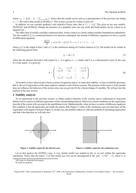
describe if the system will converge to the equilibrium or not. Mathematically, when we have a system of difference equations
this condition is that all eigenvalues are inside the unitary disk (Figure 1) while in the continuous case one must have all the
eigenvalues with negative real part (Figure 2). In this way, the problem reduces to efficient methods of calculating eigenvalues
and that is the direction we will take now.
i
−1
0
1
0
−i
Figure 1: stability region for the discrete case.
Figure 2: stability region for the continuous case.
Let us first analyse the (D,PM,L) case. A very similar model was studied in [4], so we just outline the eigenvalue
calculation. Notice that the matrix A of this model (see (5)) can be decomposed in the sum −1/2(U − I), where U is
1 DD stands for diminished discrepancy.
2 Q stands for quadratic.
Preprint MAT. 22/06, communicated on September 25 th , 2006 to the Department of Mathematics, Pontifícia Universidade Católica — Rio de Janeiro,
Brazil.