Stability analysis of the oligopoly problem and variations Bernardo ...
Stability analysis of the oligopoly problem and variations Bernardo ...
Stability analysis of the oligopoly problem and variations Bernardo ...

You also want an ePaper? Increase the reach of your titles
YUMPU automatically turns print PDFs into web optimized ePapers that Google loves.
7 The <strong>oligopoly</strong> <strong>problem</strong><br />
1<br />
β 1 β 2 β 3<br />
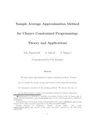
Figure 3: The graph <strong>of</strong> f(λ)<br />
Let us summarize what we have done so far. We wanted to calculate <strong>the</strong> eigenvalues <strong>of</strong> matrix A in (12). We decomposed<br />
A in a product <strong>of</strong> simpler matrices whose spectrum is equal to σ(A). Afterwards we identified this product as being a diagonal<br />
matrix E 2 minus a tensor product E½⊗E½. If we set up <strong>the</strong> eigenvalue equation (13) for this matrix we fall in <strong>the</strong> case<br />
described by equation (10). Following <strong>the</strong> same steps we did for equation (10) we arrived at (14). Defining <strong>the</strong> denominator<br />
<strong>of</strong> (14) by f(λ) we were able to conclude that <strong>the</strong> eigenvalues <strong>of</strong> <strong>the</strong> original matrix A were <strong>the</strong> zeroes <strong>of</strong> this function f(λ).<br />
Fortunately, not only <strong>the</strong> expression <strong>of</strong> f(λ) is simple but also its zeroes are located between <strong>the</strong> asymptotes β i , each one<br />
on an interval. To obtain a very good approximation <strong>of</strong> <strong>the</strong> eigenvalues <strong>of</strong> A one may use Newton’s method at each interval,<br />
with initial condition given by, for instance, <strong>the</strong> mean value <strong>of</strong> <strong>the</strong> interval (except for <strong>the</strong> first interval, <strong>of</strong> course). In <strong>the</strong> next<br />
session we will run <strong>the</strong> calculations using this procedure for a very simple example.<br />
One final remark: we have to be a little more careful when an eigenvalue <strong>of</strong> <strong>the</strong> diagonal matrix has multiplicity k, k > 1,<br />
that is, k <strong>of</strong> <strong>the</strong> diagonal entries are equal. What happens is that this eigenvalue is also an eigenvalue <strong>of</strong> <strong>the</strong> perturbation,<br />
but with multiplicity k − 1. We propose an intuitive explanation. Suppose two eigenvalues are very, very close. The <strong>the</strong>ory<br />
developed in this section tells us that <strong>the</strong>re is an eigenvalue <strong>of</strong> <strong>the</strong> perturbation between <strong>the</strong> asymptotes defined by <strong>the</strong> multiple<br />
eigenvalue <strong>and</strong> that <strong>the</strong> graph <strong>of</strong> f(λ) between <strong>the</strong>se two values is almost a vertical line. In <strong>the</strong> limit, <strong>the</strong> two asymptotes<br />
collapse <strong>and</strong> a multiple eigenvalue <strong>of</strong> <strong>the</strong> diagonal matrix arises, which is also an eigenvalue <strong>of</strong> <strong>the</strong> perturbation itself.<br />
(c) Computing <strong>the</strong> eigenvectors<br />
The hard work is to compute <strong>the</strong> approximate eigenvalues. Given <strong>the</strong>se approximations, we present two straightforward<br />
procedures to approximate <strong>the</strong> eigenvalues with high accuracy. They both can be found in [1].<br />
The first method is called Inverse Iteration. It is a variant <strong>of</strong> <strong>the</strong> well-known Power Method, where you arbitrarily choose<br />
a vector u <strong>and</strong> compute <strong>the</strong> sequence u, Au, A 2 u, . . .. It can be shown (see [1], page 154) that this sequence converges to <strong>the</strong><br />
eigenvector with <strong>the</strong> largest absolute value. In our case we want not only <strong>the</strong> eigenvector associated with <strong>the</strong> largest eigenvalue<br />
but all <strong>the</strong> eigenvalues. To do so we need to slightly modify <strong>the</strong> power method: now we compute <strong>the</strong> power sequences with<br />
matrix (A − µ) −1 instead <strong>of</strong> A. Running <strong>the</strong> calculations for an arbitrary vector u, we obtain an approximation for <strong>the</strong><br />
eigenvector associated with <strong>the</strong> eigenvalue closest to µ. As we have already approximated <strong>the</strong> eigenvalues <strong>of</strong> A, we just<br />
apply <strong>the</strong> inverse iteration with µ = ˜λ, that is, using matrix (A − ˜λ) −1 for each approximated eigenvalue ˜λ. With only a few<br />
iterations a very good approximation ṽ i <strong>of</strong> <strong>the</strong> eigenvectors is obtained, which can be verified by computing Aṽ i − ˜λ i ṽ i <strong>and</strong><br />
observing how close to zero this quantity is.<br />
Ano<strong>the</strong>r procedure is based on lemma 5.2 <strong>of</strong> [1] <strong>and</strong> is specially designed for matrices <strong>of</strong> type D + u ⊗ u, D diagonal,<br />
which is our case. The lemma states that if λ is an eigenvalue <strong>of</strong> E 2 − E½⊗E½, <strong>the</strong>n (E 2 − λI) −1 E½is <strong>the</strong> eigenvector<br />
associated to <strong>the</strong> eigenvalue λ. There is just one catch: we do not want an approximated eigenvector <strong>of</strong> E 2 − E½⊗E½<br />
but from A, <strong>and</strong> we only know that <strong>the</strong>se two matrices have <strong>the</strong> same spectrum. But we claim that if v is an eigenvector <strong>of</strong><br />
E 2 − E½⊗E½associated to <strong>the</strong> eigenvalue λ, <strong>the</strong>n Ev is an eigenvector <strong>of</strong> A. Indeed,<br />
A(Ev) = E 2 C(Ev) = E(ECE)v = E(E 2 − E½⊗E½)v = λ(Ev),<br />
where C is <strong>the</strong> matrix I −½⊗½. With this result one may easily obtain <strong>the</strong> approximated eigenvalue ṽ associated to <strong>the</strong><br />
approximated eigenvector ˜λ: first compute ũ = (E − ˜λI) −1 E½in order to obtain ṽ = Eũ.<br />
Preprint MAT. 22/06, communicated on September 25 th , 2006 to <strong>the</strong> Department <strong>of</strong> Ma<strong>the</strong>matics, Pontifícia Universidade Católica — Rio de Janeiro,<br />
Brazil.