dynamical synthesis of oscillating system mass-spring-magnet

DYNAMICAL SYNTHESIS OF OSCILLATING SYSTEM
MASS-SPRING-MAGNET
Rumen NIKOLOV, Todor TODOROV
Technical University of Sofia, Bulgaria
Abstract. On the basis of a qualitative analysis of nonlinear differential equation, which describes the behavior of the
oscillating system mass-spring-magnet, a dynamical synthesis is performed. The magnetic force is obtained using the
finite element method and approximated by an analytical expression. The parameters of the system which ensure
periodical oscillations with given properties are determined.
Keywords: nonlinear dynamics, qualitative analysis, phase portrait, separatrix, magnetic force, FEM
1. Introduction
The tasks of dynamical synthesis of mechanical
systems come down to determining of mass and
force parameters depending on preliminarily
described manner of behavior. For example, in the
Theory of Mechanisms and Machines a typical
problem of such a kind is the finding of the moment
of inertia of a flywheel, which ensures a given
irregularity of motion [1]. Tasks of the same type
concern the time-response or the durability of
transient states [2, 3].
Magneto-mechanical systems are with
sophisticated characteristics and the description of
their behavior is based on solving of nonlinear
ODEs [4, 5], and in the general case it relates to
investigation of complicated dynamical processes
which are described by PDEs [6]. The choice of the
parameters of such a system also can be added to
the tasks of the dynamical synthesis, as far as such a
choice can guarantee some requested properties of
the real system.
At the present paper a nonlinear oscillating
system of the type mass-spring-magnet is
investigated. On the basis of a qualitative analysis a
method for achieving of given parameters of the
oscillations is proposed.
2. Magnetic force determination
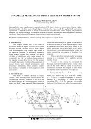
The basic elements of the system are shown in
Figure 1. Ferromagnetic mass is fixed to the free
end of cantilever and oscillates in the force field of
a permanent magnet. When the cantilever is in
undistorted shape and it is in horizontal position
between the faces of ferromagnetic mass and
magnet, an initial air gap h is established. A linear
generalized coordinate y is chosen for describing of
the mass oscillations. Zero position of this
coordinate corresponds to the horizontal position of
the cantilever.
A
Elastic cantilever
Ferromagnetic mass
B
G
F m
Fixed permanent
magnet
Figure 1. Scheme of the oscillating system
In order the oscillating system to be
qualitatively investigated, it is necessary to be
determined the force dependence on the position.
This function is worked out for any particular case
and it depends on dimensions, shape and material
properties.
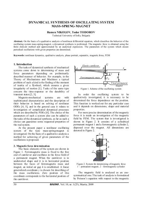
For more precise determination of the magnetic
force it is made an investigation of the magnetic
field by FEM. The system that is investigated is
shown in Figure 2. It consists of a cylindrical
permanent magnet 1 and a ferromagnetic cylinder 2,
disposed over the magnet. All dimensions are
denoted in Figure 2.
d
2
1
Figure 2. System for determining of magnetic force
1 – permanent magnet; 2 – ferromagnetic cylinder
The magnetic field is analyzed as an axesymmetrical
one. The task of analysis is formulated
by Poisson’s equation with respect to the magnetic
h c
δ
h m
y
h
x
50 RECENT, Vol. 10, nr. 1(25), Martie, 2009

Dynamical Synthesis of Oscillating System Mass-Spring-Magnet
vector-potential in the cylindrical coordinate
system. The investigated area is determined as
sufficient large buffer zone (of the order of
20-multiple dimension of the system) at the
boundary of which they are imposed homogenous
boundary conditions of Dirichlet.
The problem is solved with the help of the
software product FEMM (Finite Element Method
Magnetics), and for automation of the calculations
some programs in the Lua Script ® language are
created. For determining of the magnetic force the
built in tension tensor of Maxwell is used. The
number of mesh nodes of the finite elements varies
for the different tasks between 18,000 and 20,000.
Investigations are made for two types of
permanent magnets (BaFerrite and NDFeB) and two
dimensions of the diameters (8 and 13 mm). Results
for the magnetic field distribution and for the
attractive force between magnet and ferromagnetic
cylinder are obtained when the air gap changes from
1 to 5 mm.
Magnetic field lines for diameter 8 mm and
permanent BaFerrite for air gaps 1 and 5 mm are
visualized in Figures 3a and 3b. For the same
dimensions an investigation is made for the
permanent magnet NdFeB. Results for the magnetic
field distribution are given in Figure 3c.
As a consequence, there is no a principle
difference in the distribution field patterns of both
types of magnets. However the difference in terms
of force is significant, which can be observed in
Table 1. For the magnet of NdFeB the mean
magnetic force is more of 60 times bigger than the
same force in the system of BaFerrite.
Table 1. Force variation
Force [N]
δ [mm]
BaFerrite NdFeB BaFerrite
8/15/10 8/15/10 13/8/5
1 0.121 8.50 0.209
1.5 0.091 5.92 0.158
2 0.065 4.13 0.118
2.5 0.046 2.95 0.089
3 0.033 2.17 0.068
3.5 0.026 1.63 0.053
4 0.019 1.20 0.041
4.5 0.014 0.90 0.033
5 0.011 0.70 0.026
The obtained force data are approximated by
the relation
κ
F m =
( δ0 + δ) 2
(1)
which is close to Coulomb’s low [7] when δ 0 is
small. Analogically to this law here κ is denoted as
an imaginary magnetic mass, δ 0 is an imaginary
initial gap. The constant values and maximal
deviations are shown in Table 2. The graphs of the
approximating functions are presented in Figure 4.
c)
Figure 3. Magnetic field lines distribution for δ = 1 mm
and δ = 5 mm
а) NdFeB d = 8 mm; h m = 15 mm; h c = 10 mm;
b) BaFerrite d = 8 mm; h m = 15 mm; h c = 10 mm;
c) BaFerrite d = 13 mm; h m = 8 mm; h c = 5 mm
Table 2. Constant values and maximal deviations
Material
Max.
dimensions κ
deviation
d / h m / h c ×10 -7 [N·m 2 ] δ 0 [m] ×10 -6 [N]
BaFerrite
6.2681702 0.0012348 0.00086
8/15/10
NdFeB
35.921246 0.0010328 0.207×10 -6
8/15/10
BaFerrite
1.4354750 0.0015858 0.000124
13/8/5
3. Dynamical model of the oscillating system
A mathematical model of the beam is created,
taking in account the following more important
simplified assumptions: all kinds of resistance are
neglected; the influence of the distributions of all
kind of loads is neglected, it is assumed that the
mass moves rectilinearly and its rotation is ignored.
RECENT, Vol. 10, no. 1(25), March, 2009 51
a)
b)

F m
[N]
F m
[N]
F m
[N]
Dynamical Synthesis of Oscillating System Mass-Spring-Magnet
[mm]
[mm]
[mm]
c)
Figure 4. Approximated static characteristics of
investigated cases: а) magnet BaFerrite and dimensions
d = 8 mm; h m = 15 mm; h c = 10 mm; b) magnet NdFeB
and dimensions d = 8 mm; h m = 15 mm; h c = 5 mm;
c) magnet BaFerrite d = 13 mm; and dimensions h m = 8
mm; h c = 5 mm
According to Figure 1 for magnetic force (1) it
is yield
κ
F m =
( δ0 + h − y) 2
(2)
because δ = h – y. On the mass it exerts influence
the elastic force of the cantilever
F e = −c⋅
y
(3)
and the weight
G = m·g, (4)
where c is the spring stiffness, m is the mass, and g
is the gravity acceleration.
The motion of the mass in the free cantilever
end is described by the differential equation
κ
m ⋅ y& + c ⋅ y = m⋅
g +
(5)
( δ0
+ h − y)
which after dividing to m takes the view
κ
& y&
2
+ k ⋅ y = g +
(6)
m( δ0
+ h − y)
52 RECENT, Vol. 10, nr. 1(25), Martie, 2009
a)
b)
where k is the natural frequency of the system. For
the stroke constrains of the cantilever it follows that
y ≤ h.
After substituting h 0 = δ 0 + h, introducing
dimensionless time t new = k 2·t and change of the
variable
y = h 0 − ξ
(7)
the differential equation (6) takes the form
& β
ξ & + ξ − α +
2
ξ
= 0 . (8)
Here are denoted the following parameters
g
κ
α = h0
− ,
β = . (9)
2
2
k
m⋅ k
For the change of the variable it follows the
constrain
ξ ≥ δ 0 . (10)
By the energy transformation & ξ
ξ & 1 d 2
=
&
the
2 dξ
differential equation is yield
2
1 d ξ & β
= α − ξ −
(11)
2 dξ
2
ξ
from which after separating of the variables the first
integral is worked out
1 β
ξ & 2 1 2
= αξ − ξ + + C . (12)
2 2 ξ
By the so obtained expression after substitution
with different values of the integrating constant C
the phase trajectories in the plane ξ & , ξ of the
oscillating system can be described [8].
4. Determination of the bifurcation areas
Bifurcation zones are determined by the values
of the parameters α and β for which the phase states
of the system change its nature. For these states to
be worked out the function
1 2 β
f = α ⋅ξ − ξ + , (13)
2 ξ
is considered, which completely determines the
phase trajectories. For this purpose Eq. (13) is
presented as a sum of two functions
f = f 1 + f 2
(14)
where
1 2
β
f 1 = α⋅ ξ − ξ , f 2 = . (15)
2
ξ
From (9), β is a positive nonzero parameter but
α theoretically can be also negative and zero
parameter. The negative values of α are possible
when simultaneously the air gap h and the

Dynamical Synthesis of Oscillating System Mass-Spring-Magnet
imaginary gap δ 0 are small, and the natural
frequency k is low. Such values are relatively rarely
used in the techniques. It is known that the function
f 2 is discontinuous for ξ = 0 and it is strictly
monotone decreasing. The function f 1 is a parabola
with a zero root and a second root equal to 2α. They
are possible two variants of the sum function f. The
first one is it to be a strictly monotone decreasing
function, and the second one is it to possess two
extremes. At the first case there will not be a
singular point in the phase trajectories. At the
second case two singular points will occur, that
correspond to the stable and unstable equilibrium
points. The limit case between the two states is a
point of inflection in the function f. For this it
follows the appearance of a cusp point in the phase
trajectories. From this limit state the condition of
bifurcation is obtained, which is expressed as
simultaneously null of first and second derivation of
f. It follows to the system
β
α − ξ −
2
ξ
= 0 2β
; −1
= 0 .
3
(16)
ξ
From the system (16) it is obtained
1 β = ξ
3 ;
2
3 α = ξ ,
2
(17)
which is a parametric equation of the bifurcation
curve. After isolating of the parameter ξ the
equation of the bifurcation curve
β =
4 α
3
(18)
27
is obtained. The graph of this curve is presented in
Figure 5.
From the above mentioned it follows that for
values of α and β over the bifurcation curve, i.e.
when
4 β > α
3
(19)
27
conditions for oscillations do not exist. In case of
this combination of the parameters the mass will
accomplish only one displacement with variable
acceleration. The closer to the magnet is the mass,
the higher is its velocity. This kind of motion and
the functions f, f 1 and f 2 , are shown in Figure 6.
Vice versa, if α and β are with values under the
bifurcation curve, both oscillating or aperiodical
one-way motion are possible. This kind of motion
and the functions f, f 1 and f 2 are shown in Figure 7.
Figure 5. Bifurcation curve
Figure 6. Typical phase portraits of the system with
values of α and β over the bifurcation curve
RECENT, Vol. 10, no. 1(25), March, 2009 53

Dynamical Synthesis of Oscillating System Mass-Spring-Magnet
In order the Eq. (22) to possess three different
roots it is necessary
1 3 1
D = − β⋅α + β
2 < 0 , (24)
27 4
from where the condition is yield
4 β < α
3 . (25)
27
This result confirms again the proof that the
equilibrium points can exist only if the parameters
α and β are chosen under the bifurcation curve. In
this case there are three equilibrium points, but as it
can be seen on Figure 7, only two of them are
positive. This statement can be proved easily. The
equilibrium point with the biggest positive
coordinate is a stable center. The second positive
equilibrium point is an unstable saddle. Through it
the phase curve S passes, called separatrix. This
separatrix splits the phase plane in areas with stable
oscillations and areas with aperiodical single
displacements with variable accelerations.
Figure 7. Typical phase portraits of the system with α
and β under the bifurcation curve
5. Equilibrium point investigation
The equilibrium or singular points [5, 7, 8] of
the oscillating system follow from the system of
algebraic equations
& ξ & = 0 , ξ & = 0 . (20)
The second equation shows that the singular
points lie on the axis Оξ & . From the first equation
taking of account (8) it follows
β
− ξ + α −
2
ξ
= 0
(21)
or for ξ ≠ 0 it is yield
3
− ξ + α ⋅ξ − β = 0 . (22)
This cubic equation [9] has a discriminate
1 3 1 2
D = − β ⋅α + β . (23)
27 4
6. Dynamical synthesis of the oscillating system
The aim of the dynamical synthesis of the
magneto-mechanical system is expressed here in
finding of such combination of the parameters,
which guarantees periodic oscillations.
Firstly, a magnet couple with imaginary magnet
mass κ = 0.6268×10 -6 Nm 2 and imaginary initial
gap δ 0 =1.2348×10 -3 m according to formula (1) is
chosen. From the expressions (9) with a given
natural frequency k = 400 s –1 it is found
α = h 0 – g/k 2 = 0.004172. A mass m = 0.005 kg is
chosen and the condition (24) is checked up, finding
initially β = κ / m·k 2 = 7.924×10 -10 and after
substituting in β > 4α 3 / 27 = 1.075×10 -8 – obtaining
the necessary relation. The stiffness of the system is
found by c = m·k 2 = 800 N/m. The obtained
parameters are sufficient for choosing the rest of the
geometrical parameters and material properties.
The so chosen values do not guarantee oscillations
with the prescribed mechanical frequency,
because the system is nonlinear and in the considered
case it is proved that the natural frequency is lower
than the mechanical one. On bigger amplitudes
because of isohornity of the system the frequency
depends on the initial conditions.
The shape of the synthesized functions f, f 1 , f 2
and phase portrait of the system is shown in Figure
8. From the figure it can be seen that the system has
only one singular point corresponding to an
equilibrium point of type focus. The next
equilibrium point which is unstable gets in the zone
ξ < δ 0 and it could not be reached because of the
54 RECENT, Vol. 10, nr. 1(25), Martie, 2009

Dynamical Synthesis of Oscillating System Mass-Spring-Magnet
stroke constraint. The same is relevant to the third
equilibrium point, which is negative. The constraint
ξ ≥ δ 0 changes the nature of motion of the system
for the area inside the separatrix S, because here
constraints for the periodical motions appear and in
this way they turn in aperiodical ones.
7. Conclusion
The qualitative analysis of the considered
magneto-mechanical system allows the properties
of the system to be discovered. This analysis is a
unique mean of studying similar systems in the
cases when the differential equation is nonlinear
and cannot be solved exactly, or it leads to solutions
which cannot be analyzed. On the base of the
qualitative analysis it is possible a preliminarily
dynamical synthesis of the real oscillating system to
be achieved.
References
1. Konstantinov M.C.: Theory of mechanisms and machines.
Tehnika, Sofia, 1959, p. 493-501 (in Bulgarian)
2. Litvin, F.L.: Design of Mechanisms and Instrument
Elements. Mashinostroene, Moscow, 1973 (in Russian)
3. Levitskii, N.I.: Theory of mechanisms and machines. Nauka,
Moscow, 1979, p. 280-292 (in Russian)
4. Jordan, D.W., Smith, P.: Nonlinear ordinary differential
equations. 3 rd Ed. Oxford University Press Inc., New York,
2007, p. 2-126
5. Butenin, N.V., Nejmark, U.I., Fufaev, N.A.: Introduction in
nonlinear theory of oscillations. Nauka, Moscow, 1987, p.
5-51 (in Russian)
6. Timoshenko, S., Woinovski-Krieger, S.: Theory of Plates
and Shells. McGraw-Hill INC, New York, 1959, p. 63-76
7. Rothwell, E.J., Cloud, M.J.: Electromagnetics. CRC Press
LLC, London, 2001, p. 15-31
8. Khalil, K.H.: Nonlinear Equations. 2 nd Edition, Rmuee-HdI.
Inc, London, ISBN 0-13-P8U24-8, 1996, p. 57-88
9. Bronshtein, I.N.,·Semendyayev, K.A., Musiol, G.,·Muehlig,
H.: Handbook of Mathematics. 5 th Ed. Springer, ISBN 978-
3-540-72121-5, 2007, p. 39-43
Received in February 2009
δ 0
Figure 8. Phase portrait of the synthesized system
RECENT, Vol. 10, no. 1(25), March, 2009 55