Gerard L.G. Sleijpen, Peter Sonneveld and Martin B. van Gijzen, Bi ...

Author's personal copy
1108 G.L.G. Sleijpen et al. / Applied Numerical Mathematics 60 (2010) 1100–1114
Select an x 0
Select an ˜R0
Compute r 0 = b − Ax 0
k =−1, σ k = I,
Set U k = 0, C k = 0, ˜Rk = 0.
repeat
s = r k+1
for j = 1,...,s
u = s, Compute s = Au
β k = σ −1 ( ˜R∗
k k s)
u = u − U k β k , U k+1 e j = u
s = s − C k β k , C k+1 e j = s
end for
k ← k + 1
σ k = ˜R∗
k C k, α k = σ −1 ( ˜R∗
k k r k)
x k+1 = x k + U k α k , r k+1 = r k − C k α k
end repeat
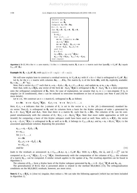
Algorithm 3. Bi-CG. 0 is the n × s zero matrix, I is the s × s identity matrix. ˜Rk is an n × s matrix such that Span( ˜Rk ) + K k (A ∗ , ˜R0 ) equals
K k+1 (A ∗ , ˜R0 ).
Example 16. ˜Rk = ¯p k (A ∗ ) ˜R0 with p k (λ) = (1 − ω k λ) ···(1 − ω 1 λ).
We will now explain how to construct a residual vector r k in K K (A, r 0 ) with K = ks + 1 that is orthogonal to K k (A ∗ , ˜R0 ).
Let C 0 be the n × s matrix with columns Ar 0 ,...,A s r 0 .ThematrixC 0 is of the form AU 0 with U 0 explicitly available:
U 0 =[r 0 ,...,A s−1 r 0 ].
Now, find a vector ⃗α 0 ∈ C s such that r 1 ≡ r 0 − C 0 ⃗α 0 ⊥ ˜R0 , r 1 ∈ K s+1 (A, r 0 ), and update x 0 as x 1 = x 0 + U 0 ⃗α 0 .
Note that, with σ 0 ≡ ˜R∗
0 C 0 any vector of the form w − C 0 σ −1
0
˜R ∗ 0 w is orthogonal to ˜R0 : I − C 0 σ −1
0
˜R 0 isaskewprojection
onto the orthogonal complement of ˜R0 . Here, for ease of explanation, we assume that σ 0 is s × s non-singular. If σ 0 is
singular (or ill conditioned), then s can be reduced to overcome breakdown or loss of accuracy (see Note 4 and [10] for
more details).
Let v = r 1 . We construct an n × s matrix C 1 orthogonal to ˜R0 as follows:
s = Av,
s = s − C 0 (σ −1
0
˜R ∗ 0 s), C 1e j = s, v = s for j = 1,...,s.
˜R ∗ 0s). Note that more stable approaches as GCR (or
1 C 1, the vector
Here, C 1 e j = s indicates that the j-column of C 1 is set to the vector s: e j is the jth (s-dimensional) standard basis
vector. Then C 1 is orthogonal to ˜R0 and its columns form a basis for the Krylov subspace of order s generated by
A 1 ≡ (I − C 0 σ −1
0
˜R ∗ 0 )A and A 1r 1 . Note that there is a matrix U 1 such that C 1 = AU 1 . The columns of U 1 can be computed
simultaneously with the columns of C 1 : U 1 e j = v − U 0 (σ −1
0
Arnoldi) for computing a basis of this Krylov subspace could have been used as well. Now, with σ 1 ≡ ˜R∗
r 2 ≡ r 1 − C 1 (σ −1
1
˜R ∗ 1 r 1) is orthogonal to ˜R0 as well as to ˜R1 ,itbelongstoK 2s+1 (A, r 0 ), and x 2 = x 1 + U 1 (σ −1
1
˜R ∗ 1 r 1) is the
associated approximate solution. Repeating the procedure
r k+1 = r k − C k ⃗α k ⊥ ˜Rk
v = r k+1
for j = 1,...,s
s = Av
C k+1 e j = s − C k
⃗β j ⊥ ˜Rk
v = C k+1 e j
end for (11)
leads to the residuals as announced: r k ∈ K ks+1 (A, r 0 ), r k ⊥ K k (A ∗ , ˜R0 ). Withσ k ≡ ˜R∗
k C k, the⃗α k and ⃗β j = ⃗β (k) can be
j
computed as ⃗α k = σ −1 ( ˜R∗
k k r k), ⃗β j = σ −1 ( ˜R∗
k k s). Simultaneously with the computation of the columns of C k+1, the columns
of a matrix U k+1 can be computed. A similar remark applies to the update of x k . The resulting algorithm can be found in
Algorithm 3.
The columns of C k+1 form a Krylov basis of the Krylov subspace generated by A k+1 ≡ (I − C k σ −1 ˜R ∗ k k )A and A k+1r k .
The generalization of Bi-CG that is presented above is related to the method ML(k)BiCG [13]. The orthogonalization
conditions on the ML(k)BiCG residuals, however, are more strict.
Note 4. If σ k = ˜R∗
k C k is (close to) singular, then reduce s. We can take the following approach (which has not been included
in Algorithm 3).