Gerard L.G. Sleijpen, Peter Sonneveld and Martin B. van Gijzen, Bi ...

Author's personal copy
1110 G.L.G. Sleijpen et al. / Applied Numerical Mathematics 60 (2010) 1100–1114
Select an x 0
Select an ˜R0
Compute r 0 = b − Ax 0
k = 0, s = r 0
for j = 1,...,s
U 0 e j = s, s = As, S 0 e j = s
end for
repeat
σ k = ˜R∗
0 S k, ⃗α k = σ −1
k
v = r k − S k ⃗α k
s = Av
Select an ω k
r k+1 = v − ω k s
for
j = 1,...,s
( ˜R∗
0 s)
⃗β j = σ −1
k
v = s − S k
⃗β j
s = Av
S k+1 e j = v − ω k s
end for
k ← k + 1
end repeat
( ˜R∗
0 r k)
Select an x
Select an ˜R0
Compute r = b − Ax
s = r
for j = 1,...,s
Ue j = s, s = As, Se j = s
end for
repeat
σ = ˜R∗
0 S, ⃗α = σ −1 ( ˜R∗
0 r)
x = x + U⃗α, v = r − S⃗α
s = Av
Select an ω
x = x + ωv, r = v − ωs
for j = 1,...,s
⃗β = σ −1 ( ˜R∗
0 s)
u = v − U ⃗β, v = s − S ⃗β
s = Av
U ′ e j = u − ωv, S ′ e j = v − ωs
end for
U = U ′ , S = S ′
end repeat
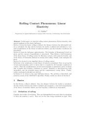
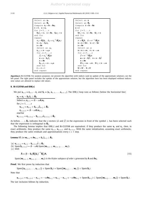
Algorithm 4. Bi-CGSTAB. For analysis purposes, we present the algorithm with indices (and no update of the approximate solution), see the
left panel. The right panel includes the update of the approximate solution, but the algorithm here has been displayed without indices:
new values are allowed to replace old values.
8. Bi-CGSTAB and IDR(s)
We put s k+1 ≡ r k+1 − r k and S k ≡[s k , s k−1 ,...,s k+1−s ].TheIDR(s) loop runs as follows (below the horizontal line)
v k = r k − S k ⃗α k ⊥ ˜R0
Select ω, r k+1 = (I − ωA)v k
for j = 1,...,s
v k+ j = r k+ j + S k+ j
⃗β k+ j ⊥ ˜R0
r k+ j+1 = (I − ωA)v k+ j
end for
v k+1+s = r k+1+s − S k+1+s ⃗α k+1+s ⊥ ˜R0
As before, ...⊥ ˜R0 indicates that the s-vectors (⃗α and ⃗β) in the expression in front of the symbol ⊥ has been selected such
that the expression is orthogonal to ˜R0 .
The following lemma implies that IDR(s) and Bi-CGSTAB are equivalent: if they produce the same v k and r k , then, in
exact arithmetic, they produce the same r k+1 , v k+s+1 and r k+1+s . With the same initialization, assuming exact arithmetic,
they produce the same residuals and approximations every s + 1step.
Lemma 17. Let w k+ j ≡ Av k+ j + S k ⃗γ k+ j ⊥ ˜R0 .
(a) v k+1+s = r k+1 − S k+1+s
⃗˜α ⊥ ˜R0 .
(b) Span(S k+1+s ) = (I − ωA) Span([w k+s−1 , w k+s−2 ,...,w k ]).
(c) With
à ≡ ( ( )
I − S k ˜R∗ 0 S −1
k
˜R∗ 0)
A, (15)
Span([w k+s−1 , w k+s−2 ,...,w k ]) is the Krylov subspace of order s generated by à and Ãv k .
Proof. We first ( prove by induction that
Span [s k+ j+1 ,...,s k+1 ] ) + Span(S k ) = ( Span [w k+ j ,...,w k ] ) + Span(S k ).
Note that
s k+ j+1 = r k+ j+1 − r k+ j =−ωAv k+ j + v k+ j − r k+ j ∈−ωAv k+ j + Span(S k+ j ) ⊂ ( Span [w k+ j ,...,w k ] ) + Span(S k ).
The last inclusion follows by induction.