Gerard L.G. Sleijpen, Peter Sonneveld and Martin B. van Gijzen, Bi ...

Author's personal copy
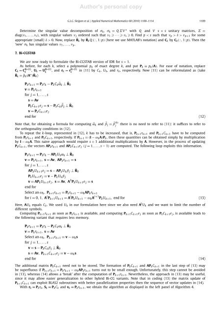
G.L.G. Sleijpen et al. / Applied Numerical Mathematics 60 (2010) 1100–1114 1109
Determine the singular value decomposition of σ k , σ k = Q Σ V ∗ with Q and V s × s unitary matrices, Σ =
diag(ν 1 ,...,ν s ), with singular values ν j ordered such that ν 1 ··· ν s 0. Find p < s such that ν p >δ>ν p+1 for some
appropriate (small) δ>0. Now, replace ˜Rk by ˜Rk Q ( : , 1: p) (hereweuseMATLAB’snotation)andC k by C k ( : , 1: p). Then the
‘new’ σ k has singular values ν 1 ,...,ν p .
7. Bi-CGSTAB
We are now ready to formulate the Bi-CGSTAB version of IDR for s > 1.
As before, for each k, select a polynomial p k of exact degree k, and put P k ≡ p k (A). For ease of notation, replace
C k = C Bi-CG , U
k k = U Bi-CG , and r
k
k = r Bi-CG in (11) by C
k
k , U k , and r k , respectively. Now (11) can be reformulated as (take
˜R k = ¯p k (A ∗ ) ˜R0 )
P k r k+1 = P k r k − P k C k ⃗α k ⊥ ˜R0
v = P k r k+1
for j = 1,...,s
s = Av
P k C k+1 e j = s − P k C k
⃗β j ⊥ ˜R0
v = P k C k+1 e j
end for (12)
Note that, for obtaining a formula for computing ⃗α k and ⃗β j = ⃗β (k) there is no need to refer to (11): it suffices to refer to
j
the orthogonality conditions in (12).
To repeat the k-loop, represented in (12), k has to be increased, that is, P k+1 r k+1 and P k+1 C k+1 have to be computed
from P k r k+1 and P k C k+1 , respectively. If P k+1 = (I − ω k A)P k , then these quantities can be obtained simply by multiplication
by I − ω k A. This naive approach would require s + 1 additional multiplications by A. However, in the process of updating
P k C k+1 , the vectors AP k r k+1 and AP k C k+1 e j ( j = 1,...,s − 1) are computed. The following loop exploits this information.
P k r k+1 = P k r k − AP k U k α k ⊥ ˜R0
v = P k r k+1 , s = Av, AP k r k+1 = s
for j = 1,...,s
AP k U k+1 e j = s − AP k U k β j ⊥ ˜R0
P k U k+1 e j = v − P k U k β j
v = AP k U k+1 e j , s = Av, A 2 P k U k+1 e j = s
end for
Select an ω k , P k+1 r k+1 = P k r k+1 − ω k AP k r k+1
for i = 0, 1, A i P k+1 U k+1 = A i P k U k+1 − ω k A i+1 P k U k+1 , end for (13)
Here, AU k equals C k .WeusedU k in our formulation here since we also need A 2 U k and we want to limit the number of
different symbols.
Computing P k+1 r k+1 as soon as P k r k+1 is available, and computing P k+1 C k+1 e j as soon as P k C k+1 e j , is available leads to
the following variant that requires less memory.
P k r k+1 = P k r k − P k C k α k ⊥ ˜R0
v = P k r k+1 , s = Av
Select an ω k , P k+1 r k+1 = v − ω k s
for j = 1,...,s
v = s − P k C k β j ⊥ ˜R0
s = Av, P k+1 C k+1 e j = v − ω k s
end for (14)
The additional matrix P k C k+1 need not to be stored. The formation of P k C k+1 and AP k C k+1 in the last step of (13) may
be superfluous if P k+1 r k+1 = P k r k+1 − ω k AP k r k+1 turns out to be small enough. Unfortunately, this step cannot be avoided
in (13), whereas (14) allows a ‘break’ after the computation of P k+1 r k+1 . Nevertheless, the approach in (13) may be useful,
since it may allow easier generalization to other hybrid Bi-CG variants. Note that in coding (13) the matrix update of
P k+1 C k+1 can exploit BLAS2 subroutines with better parallelization properties then the sequence of vector updates in (14).
With r k ≡ P k r k , S k ≡ P k C k and v k ≡ P k r k+1 , we obtain the algorithm as displayed in the left panel of Algorithm 4.