1 PHYS 1101 Practice problem set 9, Chapter 29: 6, 15, 28, 41, 52 ...
1 PHYS 1101 Practice problem set 9, Chapter 29: 6, 15, 28, 41, 52 ...
1 PHYS 1101 Practice problem set 9, Chapter 29: 6, 15, 28, 41, 52 ...

Create successful ePaper yourself
Turn your PDF publications into a flip-book with our unique Google optimized e-Paper software.
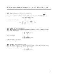
<strong>PHYS</strong> <strong>1101</strong> <strong>Practice</strong> <strong>problem</strong> <strong>set</strong> 9, <strong>Chapter</strong> <strong>29</strong>: 6, <strong>15</strong>, <strong>28</strong>, <strong>41</strong>, <strong>52</strong>, 63, 71, 79;<br />
<strong>Chapter</strong> 30: 27, 33, 57, 62, 65, 67, 68, 83<br />
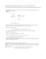
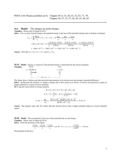
<strong>29</strong>.6. Model: The charges are point charges.<br />
Visualize: Please refer to Figure Ex<strong>29</strong>.6.<br />
Solve: For a system of point charges, the potential energy is the sum of the potential energies due to all pairs of charges:<br />
Kq i<br />
q j<br />
U elec<br />
= ∑ = U 12<br />
+ U 13<br />
+ U 23<br />
= K q q 1 2<br />
+ K q 1q 3<br />
+ K q 2<br />
q 3<br />
r 12<br />
r 13<br />
i,j<br />
r ij<br />
= ( 9.0 × 10 9 N m 2 / C 2 ⎡ ( 2 nC )( −1.0 nC ) (<br />
)<br />
+ 2 nC ) ( −1.0 nC ) ( −1 nC) + ( −1.0 nC ) ⎤<br />
⎢<br />
⎥<br />
⎣ 0.03 m<br />
0.03 m<br />
0.03 m ⎦<br />
r 23<br />
= −0.60 × 10 −6 J − 0.60 × 10 −6 J + 0.30 × 10 −6 J = −0.90 ×10 −6 J<br />
Assess: Note that U 12 = U 21 , U 13 = U 31 , and U 23 = U 32 .<br />
<strong>29</strong>.<strong>15</strong>. Model: Energy is conserved. The potential energy is determined by the electric potential.<br />
Visualize:<br />
The figure shows a before-and-after pictorial representation of an electron moving through a potential difference.<br />
Solve: (a) Because the electron is a negative charge and it slows down as it travels, it must be moving from a region of<br />
higher potential to a region of lower potential.<br />
(b) Using the conservation of energy equation,<br />
⇒ ΔV = − mv 2<br />
i<br />
2e<br />
K f + U f = K i + U i ⇒ K f + qV f = K i + qV i<br />
⇒ V f − V i = 1 (<br />
q K i − K f<br />
) =<br />
1<br />
( −e)<br />
= − 9.11 × 10<br />
−31<br />
kg<br />
2 1.60 × 10 −19 C<br />
1<br />
( 2 mv 2 i − 0 J )<br />
( )( 5.0 ×10 5 m / s) 2<br />
( )<br />
= −0.712 V<br />
Assess: The negative sign with ΔV verifies that the electron moves from a higher potential region to a lower potential<br />
region.<br />
<strong>29</strong>.<strong>28</strong>. Model: The net potential is the sum of the potentials due to each charge.<br />
Visualize: Please refer to Figure Ex<strong>29</strong>.<strong>28</strong>.<br />
Solve: From the geometry in the figure,<br />
1.5 cm 1.5 cm 1.5 cm<br />
1.5 cm<br />
= = = cos 30° ⇒ r 1 = r 2 = r 3 =<br />
r 3 cos30°<br />
The potential at the dot is<br />
r 1<br />
r 2<br />
= 1.732 cm<br />
1
V =<br />
1<br />
4πε 0<br />
q 1<br />
r 1<br />
+<br />
1<br />
4πε 0<br />
q 2<br />
r 2<br />
+<br />
1<br />
4πε 0<br />
q 3<br />
r 3<br />
( ) 2.0 × 10 −9 C<br />
= 9.0 × 10 9 N m 2 / C 2 ⎡<br />
0.01732 m − 1.0 × 10 −9 C<br />
0.01732 m − 1.0 ×10 −9 C ⎤<br />
⎣ ⎢<br />
0.01732 m ⎦ ⎥ = 0 V<br />
Assess: Potential is a scalar quantity, so we found the net potential by adding three scalar quantities.<br />
<strong>29</strong>.<strong>41</strong>. Model: Mechanical energy is conserved. Metal spheres are point particles and they have point charges.<br />
Visualize:<br />
Solve: (a) The system could have both kinetic and potential energy, although here K = 0 J. The energy of the system is<br />
E 0<br />
= K 0<br />
+ U 0<br />
= 0 J + q A q B<br />
4πε 0<br />
r 0<br />
= 9.0 ×10 9 N m 2 / C 2<br />
(b) In static equilibrium, the net force on sphere A is zero. Thus<br />
( )( 2.0 ×10 −6 C) ( 2.0 ×10 −6 C)<br />
0.05 m<br />
( )( 2.0 × 10 −6 C) ( 2.0 × 10 −6 C)<br />
= 0.720 J<br />
T = F B on A = q q A B<br />
4πε 0 r = 9.0 × 10 9 N m 2 / C 2<br />
= 14.4 N<br />
2<br />
0 ( 0.05 m ) 2<br />
(c) The spheres move apart due to the repulsive electric force between them. The surface is frictionless, so they continue to<br />
slide without stopping. When they are very far apart (r 1 → ∞), their potential energy U 1 → 0 J. Energy is conserved, so we<br />
have<br />
E 1<br />
= K 1<br />
+ U 1<br />
= 1 2<br />
2<br />
m A<br />
v A1<br />
+ 1 2<br />
2<br />
m B<br />
v B1<br />
+ 0 J = E 0<br />
Momentum is also conserved: P after = m A v A1 + m B v B1 = P before = 0 kg m/s. Note that these are velocities and that v A1 is a<br />
negative number. From the momentum equation,<br />
Substituting this into the energy equation,<br />
⇒ v B1<br />
=<br />
⎛<br />
E 0 = 1 2 m A − m v B B1<br />
⎜<br />
⎝ m A<br />
2 E 0<br />
m B m B m A +1<br />
v A1<br />
⎞<br />
⎟<br />
⎠<br />
2<br />
= − m B v B1<br />
m A<br />
+ 1 2<br />
2 m B v B1<br />
⎛ m<br />
= 1 2 m B<br />
⎞ 2<br />
B ⎜ + 1⎟ v B1<br />
⎝ m A ⎠<br />
( ) = 2( 0.720 J )<br />
( 0.004 kg )( 4 g 2 g + 1) = 10.95 m / s<br />
Using this result, we can then find v A1 = −m B v B1 m A = −21.9 m / s . These are the velocities, so the final speeds are 21.9<br />
m/s for the 2 g sphere and 10.95 m/s for the 4 g sphere.<br />
2
<strong>29</strong>.<strong>52</strong>. Model: Energy is conserved.<br />
Visualize:<br />
The dipole initially is at the higher potential energy. As it moves to its minimum energy state, the decrease in the potential<br />
energy appears as rotational kinetic energy.<br />
Solve: The potential energy of a dipole is U dipole<br />
= − p ⋅ E <br />
= − pEcosθ , where θ is the angle between the dipole and the<br />
electric field. The energy conservation equation K f + U f = K i + U i is<br />
The moment of inertia of the dipole is I dipole<br />
( )<br />
1<br />
2<br />
Iω 2 + U f<br />
= 0 J + U i<br />
⇒ 1 2<br />
Iω 2 = U i<br />
− U f<br />
= −pE cos90° − − pEcos 0°<br />
ω =<br />
2( qs)E<br />
( ) 2 =<br />
2m 1 2<br />
s<br />
⇒ 1 2<br />
Iω 2 = pE ⇒ ω =<br />
2 pE<br />
I<br />
= 2 m( 1 2 s) 2 . Substituting into the above equation,<br />
( ) 0.10 m<br />
( 1.0 ×10 −3 kg) 0.10 m<br />
4 2.0 ×10 −9 C<br />
( )( 1000 V / m)<br />
= 0.<strong>28</strong>3 rad / s<br />
( ) 2<br />
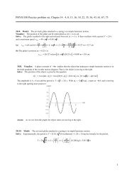
<strong>29</strong>.63. Model: The potential at any point is the superposition of the potentials due to all charges. Outside a uniformly<br />
charged sphere, the electric potential is identical to that of a point charge Q at the center.<br />
Visualize: Please refer to Figure P<strong>29</strong>.63. Sphere A is the sphere on the left and sphere B is the one on the right.<br />
Solve: The potential at point a is the sum of the potentials due to the spheres A and B:<br />
V a<br />
= V A at a<br />
+ V B at a<br />
=<br />
1<br />
4πε 0<br />
Q A<br />
R A<br />
+<br />
1<br />
4πε 0<br />
= ( 9.0 × 10 9 N m 2 / C 2<br />
) 100 × 10 −9 C<br />
0.30 m<br />
= 3000 V + 321 V = 3321 V<br />
Q B<br />
0.70 m<br />
+ ( 9.0 × 10 9 N m 2 / C 2<br />
) 25 × 10 −9 C<br />
0.70 m<br />
Similarly, the potential at point b is the sum of the potentials due to the spheres A and B:<br />
V b = V B at b + V A at b =<br />
1<br />
4πε 0<br />
( )<br />
= 9.0 × 10 9 N m 2 / C 2<br />
Q B<br />
R B<br />
+<br />
= 4500 V + 947 V = 5447 V<br />
1<br />
4πε 0<br />
Q A<br />
0.95 m<br />
⎛ 25 ×10 −9 C<br />
0.05 m + 100 ×10 −9 C⎞<br />
⎜<br />
⎟<br />
⎝<br />
0.95 m ⎠<br />
Thus, the potential at point b is higher than the potential at a. The difference in potential is V b – V a = 5447 V –<br />
3321 V = 2126 V.<br />
Assess: V A at a = 3000 V and the sphere B has a potential of 225 V at point a. The spherical symmetry dictates that the<br />
potential on a sphere’s surface be the same everywhere. So, in calculating the potential at point a due to the sphere B we<br />
used the center-to-center separation of 1.0 m rather than a separation of 100 cm – 30 cm = 70 cm from the center of sphere<br />
B to the point a. The former choice leads to the same potential everywhere on the surface whereas the latter choice will<br />
lead to a distribution of potentials depending upon the location of the point a. Similar reasoning also applies to the<br />
potential at point b.<br />
3
<strong>29</strong>.71. Model: Because the rod is thin, assume the charge lies along the semicircle of radius R.<br />
Visualize: Please refer to Figure P<strong>29</strong>.71. The bent rod lies in the xy-plane with point P as the center of the semicircle.<br />
Divide the semicircle into N small segments of length Δs and of charge ΔQ = ( Q πR)Δs , each of which can be modeled as<br />
a point charge. The potential V at P is the sum of the potentials due to each segment of charge.<br />
Solve: The total potential is<br />
V = ∑ V i =<br />
i<br />
1<br />
i<br />
∑ 4πε 0<br />
ΔQ<br />
R = 1<br />
4πε 0<br />
R<br />
⎛ Q ⎞<br />
⎝ πR ⎠ Δs 1 Q<br />
1 Q<br />
∑ =<br />
RΔθ<br />
i<br />
4πε 0<br />
∑ =<br />
πR 2<br />
i<br />
4πε 0<br />
∑ Δθ .<br />
πR<br />
i<br />
All of the terms come to the front of the summation because these quantities did not change as far as the summation is<br />
concerned. The summation does not have to convert to an integral because the sum of all the Δθ around the semicircle is π.<br />
Hence, the potential at the center of a charged semicircle is<br />
1 Qπ<br />
V center =<br />
4πε 0<br />
πR = 1 Q<br />
4πε 0<br />
R<br />
<strong>29</strong>.79. Model: Energy and momentum are conserved.<br />
Visualize: Please refer to Figure CP<strong>29</strong>.79. Let the two spheres have masses m A and m B , and speeds v A and v B when they<br />
are very far apart.<br />
Solve: The energy conservation equation K f + U f = K i + U i is<br />
⇒ 1 2<br />
2<br />
( 0.002 kg )v A<br />
1 2<br />
2<br />
m A<br />
v A<br />
+ 1 2<br />
( 2<br />
m B<br />
v B ) + 0 J = 0 J +<br />
+ 1 2<br />
2<br />
( 0.001 kg )v B<br />
1<br />
4πε 0<br />
= 9.0 ×10 9 N m 2 / C 2<br />
q A<br />
q B<br />
r AB<br />
(<br />
( ) 2.0 × 10 −9 C) ( 1.0 ×10 −9 C)<br />
⇒ v A 2 + 0.5 v B 2 = 0.0090 m 2 / s 2<br />
2.0 ×10 −3 m<br />
To solve for v A and v B , we need another equation relating v A and v B . From the momentum conservation equation P after =<br />
P before we get<br />
m A v A + m B v B = 0 kg m/s ⇒ (2.0 g)v A + (1.0 g)v B = 0 kg m/s ⇒ v B = −2v A<br />
Substituting this expression into the energy conservation equation,<br />
v A<br />
2<br />
+ 0.5( 2v A<br />
) 2 = 0.009 m 2 / s 2 2<br />
⇒ 3v A<br />
= 0.009 m 2 / s 2<br />
Solving these equations, we get v A = –0.0548 m/s and v B = +0.110 m/s. Thus the speeds are 0.0548 m/s for A and 0.110<br />
m/s for B.<br />
30.27. Visualize: Please refer to Figure Ex30.27.<br />
Solve: Any two electrodes, regardless of their shape, form a capacitor whose capacitance is defined as C = Q ΔV C<br />
. The<br />
capacitance is<br />
−9<br />
20 ×10 C<br />
C =<br />
100 V<br />
= 2.0 ×10 −10 F = 200 pF<br />
4
30.33. Solve: (a) From Equation 30.33, the energy stored in the charged capacitor is<br />
U C<br />
= 1 2 C ΔV C<br />
= 1 2<br />
( ) 2 = 1 2<br />
⎛<br />
⎝<br />
Aε 0<br />
d<br />
⎞<br />
⎠ ΔV C<br />
( ) 2<br />
( )<br />
0.50 ×10 −3 m<br />
π( 0.01 m ) 2 8.85 ×10 −12 C 2 / N m 2<br />
(b) From Equation 30.35, the energy density in the electric field is<br />
u E = 1 2 ε 0E 2 = 1 2 ε ⎛<br />
0<br />
⎝<br />
ΔV C<br />
d<br />
⎞<br />
⎠<br />
2<br />
( )<br />
= 1 2 8.85 ×10 −12 C 2 / N m 2<br />
( 200 V ) 2 = 1.11 × 10 −7 J<br />
⎛ 200 V ⎞<br />
⎝ 0.5 ×10 −3 m ⎠<br />
2<br />
= 0.708 J / m 3<br />
30.57. Model: Capacitance is a geometric property of two electrodes.<br />
Visualize:<br />
Solve: The ratio of the charge to the potential difference is called the capacitance: C = Q ΔV C<br />
. The potential difference<br />
across the capacitor is<br />
Using R 2 = R 1 + 1.0 mm,<br />
ΔV C<br />
=<br />
⎡ 1<br />
⇒ C = 4πε 0 − 1 ⎤<br />
⎢ ⎥<br />
⎣ ⎢ R 1 R 2 ⎦ ⎥<br />
1<br />
4πε 0<br />
−1<br />
Q<br />
R 1<br />
−<br />
1<br />
4πε 0<br />
Q<br />
R 2<br />
=<br />
Q ⎡ 1<br />
− 1 ⎤<br />
⎢ ⎥<br />
4πε 0 ⎣ ⎢ R 1 R 2 ⎦ ⎥<br />
= 4πε 0<br />
R 1<br />
R 2<br />
R 2 − R 1<br />
= 4πε 0<br />
R 1<br />
R 2<br />
1.0 ×10 −3 m = 100 ×10 −12 F<br />
⇒ R 1<br />
R 2<br />
= ( 100 × 10 −12 F) ( 1.0 ×10 −3 m) ( 9.0 ×10 9 N m 2 / C 2<br />
) = 900 × 10 −6 m 2<br />
( ) = 900 ×10 −6 m ⇒ R 1 2 + 1.0 × 10 −3 m<br />
R 1<br />
R 1<br />
+1.0 × 10 −3 m<br />
⇒ R 1<br />
=<br />
−1.0 ×10 −3 m ± ( 1.0 × 10 −3 m) 2 + 3600 ×10 −6 m 2<br />
2<br />
( )R 1<br />
− 900 ×10 −6 m = 0<br />
= 0.0<strong>29</strong>5 m = 2.95 cm<br />
The outer radius is R 2 = R 1 + 0.001 m = 0.0305 m = 3.05 cm. So, the diameters are 5.90 cm and 6.10 cm.<br />
30.62. Visualize:<br />
The pictorial representation shows how to find the equivalent capacitance of the three capacitors shown in the figure.<br />
Solve: Because C 1 and C 2 are in parallel, their equivalent capacitance C eq 12 is<br />
Then, C eq 12 and C 3 are in series. So,<br />
C eq 12 = C 1 + C 2 = 20 µF + 60 µF = 80 µF<br />
5
1<br />
C eq<br />
=<br />
1<br />
C eq 12<br />
+ 1 C 3<br />
=<br />
30.65. Model: Assume the battery is an ideal battery.<br />
Visualize:<br />
1<br />
80 µF + 1<br />
10 µ F = 9 ( 80 µF)<br />
−1 ⇒ C eq = 80<br />
9 µF = 8.9 µF<br />
The pictorial representation shows how to find the equivalent capacitance of the three capacitors shown in the figure.<br />
Solve: Because C 2 and C 3 are in series,<br />
C eq 23 and C 1 are in parallel, so<br />
1<br />
C eq 23<br />
= 1 C 2<br />
+ 1 C 3<br />
=<br />
1<br />
4 µF + 1<br />
6 µF = 10 ( 24 µF)<br />
−1 ⇒ C eq 23<br />
= 24<br />
10<br />
µF = 2.4 µ F<br />
C eq = C eq 23 + C 1 = 2.4 µF + 5 µF = 7.4 µF<br />
A potential difference of ΔV C = 9 V across a capacitor of equivalent capacitance 7.4 µF produces a charge<br />
Q = C eq ΔV C = (7.4 µF)(9 V) = 66.6 µC<br />
Because C eq is a parallel combination of C 1 and C eq 23 , these capacitors have ΔV 1<br />
= ΔV eq 23<br />
= ΔV C<br />
= 9 V. Thus the charges<br />
on these two capacitors are<br />
Q 1 = (5 µF)(9 V) = 45 µC Q eq 23 = (2.4 µF)(9 V) = 21.6 µC<br />
Because Q eq 23 is due to a series combination of C 2 and C 3 , Q 2 = Q 3 = 21.6 µC. This means<br />
ΔV 2<br />
= Q 21.6 µC<br />
2<br />
= = 5.4 V ΔV 3<br />
= Q 21.6 µC<br />
3<br />
=<br />
C 2<br />
4 µF<br />
C 3<br />
6 µF = 3.6 V<br />
In summary, Q 1 = 45 µC, V 1 = 9 V; Q 2 = 21.6 µC, V 2 = 5.4 V; and Q 3 = 21.6 µC, V 3 = 3.6 V.<br />
30.67. Model: Capacitance is a geometric property.<br />
Visualize: Please refer to Figure P30.67. Shells R 1 and R 2 are a spherical capacitor C. Shells R 2 and R 3 are a spherical<br />
capacitor C′. These two capacitors are in series.<br />
Solve: The ratio of the charge to the potential difference is called the capacitance:C = Q ΔV C<br />
. The potential differences<br />
across the capacitors C and C′ are<br />
ΔV C<br />
=<br />
ΔV C ′ =<br />
1<br />
4πε 0<br />
1<br />
4πε 0<br />
Q<br />
R 1<br />
−<br />
Q<br />
R 2<br />
1<br />
4πε 0<br />
1<br />
−<br />
4πε 0<br />
Q<br />
R 2<br />
=<br />
Q<br />
R 3<br />
=<br />
Q ⎡ 1<br />
− 1 ⎤<br />
⎢ ⎥<br />
4πε 0 ⎣ ⎢ R 1 R 2 ⎦ ⎥<br />
Q ⎡ 1<br />
− 1 ⎤<br />
⎢ ⎥<br />
4πε 0 ⎣ ⎢ R 2 R 3 ⎦ ⎥<br />
( )<br />
⇒ C = 4πε 0<br />
⎛ 1<br />
− 1 ⎞<br />
⎜ ⎟<br />
⎝ R 1<br />
R 2<br />
⎠<br />
−1<br />
( )<br />
C ′ = 4πε 0<br />
⎛ 1<br />
− 1 ⎞<br />
⎜ ⎟<br />
⎝ R 2<br />
R 3<br />
⎠<br />
−1<br />
Because these two capacitors are in series,<br />
1<br />
= 1 C net<br />
C + 1 C ′<br />
1 ⎛ 1<br />
= − 1 + 1 − 1 ⎞ 1 ⎛ R<br />
⎜<br />
⎟ =<br />
3<br />
− R 1<br />
⎞<br />
⎜ ⎟<br />
4πε 0<br />
⎝ R 1<br />
R 2<br />
R 2<br />
R 3<br />
⎠ 4πε 0<br />
⎝ R 1<br />
R 3<br />
⎠<br />
( )( 0.03 m )<br />
⎛ R<br />
C net<br />
= 4πε<br />
1<br />
R 3<br />
⎞<br />
1 ⎡ 0.01 m ⎤<br />
0 ⎜ ⎟ =<br />
⎢<br />
⎥ = 1.67 ×10 −12<br />
⎝ R 3<br />
− R 1<br />
⎠ 9.0 × 10 9 N m 2 / C 2 ⎣ 0.03 m − 0.01 m ⎦<br />
Assess: C net depends on only the inner and outer shells, not on R 2 .<br />
F = 1.67 pF<br />
6
30.68. Model: Assume the battery is ideal.<br />
Visualize:<br />
The circuit in Figure P30.68 has been redrawn to show that the six capacitors are arranged in three parallel combinations,<br />
each combination being a series combination of two capacitors.<br />
Solve: (a) The equivalent capacitance of the two capacitors in series is 1 2 C . The equivalent capacitance of the six<br />
capacitors is 3 2 C .<br />
(b) As points a and b are midpoints of identical capacitors, V a = V b = 6.0 V. Therefore, the potential difference between<br />
points a and b is zero.<br />
30.83. Visualize:<br />
Solve: The charge density inside the cylinder is ρ. Consider a Gaussian surface with a radius r inside the cylinder. The<br />
charge enclosed by this closed surface is Q enclosed = (πr 2 L)ρ. Using Gauss’s law,<br />
<br />
∫ E ⋅ dA<br />
<br />
= E( 2πrL ) = Q (<br />
enclosed<br />
= πr 2 L)ρ<br />
⇒ E = πr 2 Lρ<br />
ε 0<br />
ε 0 2πrL = ⎛ ρ ⎞<br />
⎜ ⎟ r ⇒ ⎛ ρ ⎞<br />
E = ⎜ ⎟ rˆ r<br />
⎝ 2ε 0 ⎠ ⎝ 2ε 0 ⎠<br />
ε 0<br />
In the last step, we have taken into account the radial direction of the electric field pointing outward. The potential<br />
difference between the surface and the axis is<br />
ΔV = −<br />
∫<br />
E <br />
⋅ dr<br />
= −<br />
R<br />
∫<br />
0<br />
ρ<br />
r ˆ r ⋅ dr = −<br />
2ε 0<br />
R<br />
∫<br />
0<br />
ρ<br />
2ε 0<br />
r dr<br />
= −ρ r 2 R<br />
= − ρR2<br />
2ε 0 2 0<br />
4ε 0<br />
7