A Sharp Interface Cartesian Grid Method for Simulating Flows with ...

More documents

Recommendations

Info

356 UDAYKUMAR ET AL. this deficit correction is applied in the problems involving the moving indentation and the diaphragm-driven pump as presented under Results, Sections 3.2 and 3.4, respectively. In the case of the oscillating cylinder problem in Section 3.3, no net efflux of mass results at the moving boundary and hence the moving boundary does not have any impact on global mass conservation. It is worth pointing out that the form of Eqs. (12) and (13) is virtually identical to (3) and (5). The primary difference is that for the trapezoidal boundary cells, the cell volume, surface area, and directions of the surface normals are now functions of time. Furthermore, the boundary conditions have to be reformulated in order to account for the time-dependant motion of the immersed boundary. However, unlike Lagrangian methods, time derivatives of the cell volume and surface area do not appear in the equation. In this respect, the simplicity of the Eulerian approach is retained. In the context of the current method, this implies that the discretization of Eqs. (12) and (13) at any given time step is virtually identical to the stationary boundary case. Thus, the spatial discretization methodology described in Section 2.2 can be used even with moving boundaries. The primary difficulty in the moving boundary algorithm comes from the appearance of “freshly cleared” cells (this issue is discussed in the next section). 2.4. “Freshly Cleared” Cells In sharp interface methods, such as the present one or those presented by Bayyuk et al. [4] and Leveque and co-workers [5, 27], the issue of change of material needs to be addressed. 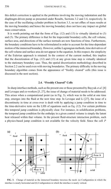This arises when a computational point (as in Fig. 3), which was in the solid at one time step, emerges into the fluid at the next time step. In Leveque and Li [27], the issue of a discontinuity in time at cross-over is dealt with by applying a jump condition in time to the time-derivative term on the LHS of equations such as Eq. (12). For certain problems this temporal jump condition is physically clear. For instance, in solidification problems, the temporal jump condition for the enthalpy in a given control volume is simply the latent heat released within that volume. In the present fluid-structure interaction problem, such a physics-based jump condition is not available for the velocity field. Since the cell P FIG. 3. Change of material as the immersed boundary traverses the mesh. (a) Configuration in which the interface is nearly horizontal and (b) Configuration in which the interface is nearly vertical.
SHARP INTERFACE CARTESIAN GRID METHOD 357 was previously in the solid and it had no history in the fluid phase, there is no physically realizable value of ⃗u i, t j . Thus, Eq. (14) is not applicable for such cells. In the current method, an approach similar to that used in the finite-difference method of Udaykumar et al. [48] is employed. This consists of temporarily merging the freshly cleared cell with a neighboring cell and is analogous to the approach taken in moving grid formulations when a new cell is inserted following mesh refinement. In the current finitevolume-based methodology, this cell-merging is realized through a simple one-dimensional interpolation operation and this can be explained here for the particular freshly cleared cell shown in Fig. 3a. For this cell, the following interpolant is used, u ∗ (y) = a 0 + a 1 y + a 2 y 2 , (16) where, the coefficients a 0 , a 1 , and a 2 are coefficients that depend on the value of ⃗u ∗ at P, N, and the boundary location B, and the corresponding locations of these points. A similar procedure can be followed for the situation illustrated in Fig. 3b. The above dependence can therefore be recast in the form ∑ = 0, (17) M B P M u∗ M and for this cell, Eq. (17) replaces the discretized advection–diffusion equation (12). Note that Eq. (17) is applied only at the instant when there is a crossover. Following that instant, Eq. (12) is again used to time step the ⃗u ∗ field. Note also that since pressure depends only on the ⃗u ∗ field, Eq. (13) is still valid for these cells as long as ⃗u ∗ can be computed through some appropriate means, such as Eq. (17). 2.5. Fast Solution of Discretized Equations The general form of the discretized equations to be solved at each time step is given in (10). The term on the left-hand side of this equation represents a discretized Helmholtz operator in the case of the advection–diffusion equation and a Laplacian operator in the case of the pressure Poisson equation. The standard alternating-direction line successive–overrelaxation (SOR) proves extremely effective for the solution of the discretized advection–diffusion equation and the residual can be reduced to acceptable levels within a few iterations. However, the discretized pressure Poisson equation (PPE) exhibits significantly slower convergence. In fact, due to its slow convergence, the solution of the discretized pressure equation is usually the most time-consuming part of a fractional-step algorithm. In the presence of immersed boundaries, this behavior of the pressure equation can be further exacerbated since the discrete operator for the trapezoidal cells requires a stencil that has significant dependence on neighbors which are not included in the line-SOR sweeps. For example, in Fig. 2c the coupling of the cell with its northeast and southwest neighbor is not included directly in any of the line-sweeps. Furthermore, discretization in the irregularly shaped boundary cells results in weaker diagonal dominance than in the regular cells and this has a deleterious effect on the convergence of any iterative scheme. In Ye et al. [58], a line-SOR preconditioned BiCGSTAB iterative method was employed and was found to be significantly faster than a simple line-SOR algorithm. Furthermore, for the stationary boundary problems that were simulated there, it was found that this iterative method allowed us to obtain the solution of most problems in a reasonable amount
Page 1 and 2: Journal of Computational Physics 17
Page 3 and 4: SHARP INTERFACE CARTESIAN GRID METH
Page 11: SHARP INTERFACE CARTESIAN GRID METH

A Sharp Interface Cartesian Grid Method for Simulating Flows with ...

Create successful ePaper yourself

Delete template?

Save as template?