Force Control with a Kalman Active Observer Applied ... - ISR-Coimbra

Paper
Force Control with a Kalman Active Observer Applied in a Robotic Skill
Transfer System*
Rui Cortesão Ý , Ralf Koeppe Þ , Urbano Nunes Ý and Gerd Hirzinger Þ
Abstract: The article describes the design of a force controller for a position-based manipulator with arbitrary
dead-time applying Kalman Active Observers. The design is based on pole placement using discrete state space
theory. An active state variable is introduced to compensate non linearities and parameter variations during the
control process. Only the output of the plant is measured. All the discrete state space is estimated using Kalman
based techniques. The robustness of the system is accomplished through optimal noise processing embedded in
the control strategy. The design was tested as a force controller in a skill transfer system at the DLR.
Keywords: Kalman Active Observers, Force Control, Stochastic Signals
1. Introduction
NO wadays the robotic technology is highly sophisticated.
Many robotic manipulators are specially designed
for a particular task, with software and hardware oriented
tools to accomplish a certain goal. If any of the system
components needs to be changed, serious problems can
result to attain the desired performance indexes for a given
task. Robot upgrades, including new robot specifications
with new sensors, often imply non-trivial changes in the
design issues, demanding efforts very Human-Power and
time consuming. To overcome these obvious drawbacks,
different strategies ought to be pursued. Modular and compliant
design, with a natural plasticity to accommodate different
specifications and set-ups is a key requirement. In
robotics there is still a lack of systematic methodologies to
develop robust intelligent architectures. The bottom layers
of these architectures deal with raw data processing, sensor
fusion, and control. The paper focus attention in a force
control module inserted in an intelligent control architecture.
The procedure here presented can be generalised for
other sensors, creating a solid platform to emerge highlevel
intelligent algorithms.
Any task that requires physical contact between the
robot and the environment needs not only a position control,
but also a control of the force exerted by the robot’s
end effector on an object [19]. Typical tasks that require
force control are the classical peg-in-hole insertion, grasping/handling
objects, and deburring. These tasks, usually
slow, are well controlled by a positional servo system. In
many robotic workstations, force feedback is implemented
as an external loop that modifies the reference input of a
position or a velocity servo system [11]. Thus, the desired
impedance of a manipulator is defined, specifying the commanded
position or velocity as a function of the force. A
£ Received February 5, 2000; accepted April 17, 2000. This work was
partially supported by Fundação Ciência e Tecnologia, project number
MENTOR PRAXIS/P/EEI/13141/1998.
Ý University of Coimbra, Institute of Systems and Robotics (ISR), 3030
Coimbra, Portugal. E-mail: cortesao, urbano@isr.uc.pt
Þ German Aerospace Center (DLR), Institute of Robotics and Mechatronics,
82230 Wessling, Germany. E-mail: Ralf.Koeppe,
Gerd.Hirzinger@dlr.de
key requirement for any force-based task is the ability to
regulate the interaction force between the manipulator and
the environment, i.e., the compliance. Large compliance
imply that a position error causes a small change in the
interaction force. Some manipulators use a compliant mechanical
element placed in the manipulator’s wrist, helping
to control forces exerted in the environment. In the literature,
there are essentially two methods used for force
control: implicit force control and explicit force control
[9]. The former consists in controlling the end-effector
forces through actuator commands. This method can only
be used for lightweight direct-drive manipulator arms, or if
the friction in the gear train of the drives is small. The latter
method also known by active force feedback, is based
on force feedback using a wrist force sensor. The main
problem of the classical force control design is its blindness
to the noises present in the whole system. In fact,
the quantification of the noises never enters in the design
issues. Demanding tasks, like peg-in-hole insertion with a
tight clearance, can become instable or suffer from residual
oscillations if the noises are not properly handled. In this
context, noises represent not only system and measurement
noises, but also parameter mismatches, non-linear effects,
discretization errors, etc. Basically they represent the difference
between the “model plant” used in the control design
and the “real plant”. Stochastic techniques should be
applied in order to handle the noises in a robust and optimal
way. The proposed force controller is designed in a systematic
way, with potential to perform parallel force/velocity
control, on-line impedance matching and robustness between
contact and non-contact states. System and measurement
noise models are obtained in a straightforward way.
State space theory and Kalman filter theory are used to design
the controller. The position response of the robot and
its associated dead-time are handled in the force control
design.
2. State Space Design
Surprisingly, most of the force control design available
in the literature is based on classical output feedback using
root locus, Bode, or Nyquist plots [16]. This design philosophy
is very far from the potentialities of the state space
c­2000 Cyber Scientific Paper No. 0xxx–YYYY/99/010020-01

desired
velocity
½
×
desired
position
Fig. 1
×Ì
½·Ì Ô×
end-effector
position
System Plant.
based control. To point out some advantages of state space
control:
¯ Easy conversion between continuous and discrete state
spaces, keeping the same state space representation.
¯ N-dimensional pole placement control. Any desired
poles in the z-plane can be reached in a straightforward
way, using Ackermann’s formula. Thus, an N-
dimensional state space system can be designed to
have any second order behaviour. The other Æ ¾
poles can be “mapped” in Þ ¼, to represent the delay.
¯ The state-space structure is very suited for state observers,
like the Kalman observer. Thus, in many
cases it is possible to have full control of the system
reading only the output of the plant.
¯ Arbitrary system dead-times are handled in a systematic
way. There is no need to re-design the synthesis
procedure if the system dead-time changes.
¯ Disturbances, non-linear effects, and parameter variations
can be merged to an extended state, enabling the
overall system to have always a state space representation.
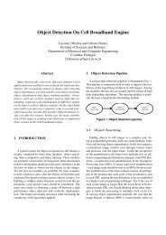
2. 1 System Plant
The position interface of industrial robots normally provides
a Cartesian decoupled behaviour to the robot’s end
effector. For each degree of freedom, the position response
is of the type [10]:
Ô´×µ
à ×
force
½
½·Ì Ô × ×Ì (1)
where the time delay Ì is due to the signal processing of
the cascade controller and has a key role in the discrete state
dimension. Ì Ô is the position response time constant. A
block diagram of the plant for each Cartesian dimension is
given in Figure 1. Ã × represents the stiffness of the system,
i.e.,
½
à ×
½
à Û
·
½
Ã
(2)
with Ã Û and à the stiffnesses of the wrist sensor and environment
respectively. For a rigid environment, Ã ½,
giving Ã × Ã Û . Hence, the plant model seen by the controller
has this form:
Ô´×µ
à ×
×´½ · Ì Ô ×µ ×Ì (3)
2. 1. 1 Discretization Procedure Given the plant
½
´×µ
×´× · Ô ×Ø (4)
½ µ
the representation in form of Equation (3) is obtained by
substituting
½ Ã × Ì Ô Ô ½ ½Ì Ô Ò Ø Ì (5)
Its equivalent temporal representation is given by
ĐÝ · Ô ½ Ý ½ Ù´Ø Ø µ (6)
where Ý is the plant output (force), and Ù is the plant input
(velocity). Defining the state variables as Ü ½ Ý and Ü ¾
Ý, Equation (6) can be written in state space form as
Ü ½ ¼ ½ ܽ
Ü ¾ ¼ Ô ½ Ü ¾
which is of the form
·
¼
½
Ù´Ø Ø µ (7)
Ü Ü´Øµ ·Ù´Ø Ø µ (8)
Physically, Ü ½ represents the force at the robot’s end effector,
and Ü ¾ its derivative. Discretizing the system of
Equation (8) with sampling time and dead-time Ø
´ ½µ · ¼ , with ¼ ¼ , the equivalent discrete
time system of Equation (9) is obtained,
¾ ¿ ¾
¿ ¾ ¿
Ü
¨ ½ ¼ ¡¡¡ ¼ Ü ½
Ù
¼ ¼ ½ ¡¡¡ ¼
Ù ½
.
. . .
.
.
. . . ..
. .
.
.
Ù ¾
¼ ¼ ¼ ¡¡¡ ½ Ù ¿
Ù ½ ¼ ¼ ¼ ¡¡¡ ¼ Ù ¾
¾ ¿
·
¼
¼
.
¼
½
Ù
½ (9)
where ¨, ¼ and ½ are given by Equations (10) to (12)
respectively [1].
¼
¨ ´µ (10)
¼
¼
½ ´ ¼ µ
´µ Ò (11)
¼
¼
´µ (12)
From Equation (8), the Laplace Transform of the state transition
matrix ¨´×µ is
¨´×µ ´×Á µ ½ (13)
¿
Using Equation (7),
¾
¼ × · Ô ½
¨´×µ ½
Computing the matrix inverse,
¾
¨´×µ ½ ×
¼
where its temporal equivalent is
¾
´Øµ
½
¿
½
×´×·Ô ½µ
½
×·Ô ½
½ ½ Ô ½ Ø
Ô ½
¼ Ô ½Ø
(14)
(15)
¿
(16)
Knowing ´Øµ from Equation (16), the computation of the
matrices ¨, ¼ and ½ is straightforward.
c­2000 Cyber Scientific Machine Intelligence & Robotic Control, 2(2), 19–27 (2000)

2. 2 Pole Placement
Equation (9) is of the form Ü ¨Ü ½ · Ù ½ . The
control design is based on pole placement using feedback
of the state variables. To accomplish a second order system
with desired damping and natural frequency Û Ò , the
characteristic polynomial of the closed loop system should
be of form
× ¾ ·¾Û Ò × · ÛÒ ¾ (17)
in the continuous domain. Its discrete representation is
given by
Þ ´Þ ¾ · ½ Þ · ¾ µ (18)
where Þ represents the delay due to the dead-time. The
parameters ½ and ¾ are computed from:
Ô
½ ¾ ÛÒ Ó×´ ½ ¾ Û Ò µ (19)
¾ ¾ÛÒ (20)
Since the system is controllable, the pole placement design
can be easily achieved using Ackermann’s formula. Hence,
the feedback gains Ä are given by
¢
£
Ä ¼ ¡¡¡ ¼ ½ Ï
½
È ´¨µ (21)
where Ï is the reachability matrix,
¢
Ï ¨ ¡¡¡ ¨Ò ½ £ (22)
Ò is the number of states, that is Ò ·¾, and È ´¨µ is
the characteristic polynomial in ¨,
È ´¨µ ¨·¾ · ½¨·½ · ¾¨
(23)
In a real physical system it is impossible to measure all
the states. Furthermore, there is always noise present in
the system due to modeling and quantization, as well as
measurement noises present in the sensors. To minimise
these problems, a Kalman Active Observer was developed
that estimates the state based on the output of the plant. The
concept of Active Observers is introduced in [5].
2. 3 Kalman Algorithm
There are many textbooks covering the Kalman filter
subject. Some well known textbooks include Gelb [8],
Jazwinski [12], Sorenson [18], and Maybeck [14]. In this
paper it is used the Bosic [2] notation for the Kalman algorithm,
in which Ü denotes the estimate of the state vector
Ü based on information up to and including time .
A generic system is represented in a state-space form by
Ü ¨ Ü ½ · Ö ½ · (24)
where the state Ü , corrupted by the system noise ,is
extracted from a noisy measurement vector Ý given by
Ý Ü · (25)
The best estimate of the state Ü , Ü , is computed from
Equations (26) to (29), which constitute the Linear Kalman
Filter for that system [6], [2].
Estimator:
Ü ¨ Ü ½ · Ö ½
·Ã Ý ´¨ Ü ½ · Ö ½ µ℄ (26)
Filter Gain:
Ã È ½ Ì È ½ Ì · Ê ℄
½
(27)
where
È ½ ¨È ½ ¨Ì · É (28)
Error Covariance Matrix:
È È ½ Ã È ½ (29)
É is the system noise matrix. Its values are function of
the properties of the system noise , É Ì .
Ê is the measurement noise matrix and is function of the
measurement noise , Ê Ì . The open loop
and the closed loop system matrices are given by ¨ and
¨ ´¨ ĵ respectively. The vector Ö is the reference
signal. The inclusion of ¨ in the observer Equation (26) is
of capital importance, permitting the reference signal Ö ½
to be the input to the observer as explained in [5].
2. 3. 1 Extended System Following the procedure of [5],
the discrete model given by Equation (9) is represented in
extended form as
¾ ¾
¿ ¾
Ü
¨ ½ ¼ ¡¡¡ ¼ ¼ Ü ½
¿
Ù
.
.
Ù ¾
Ù ½
Ô
·
¼ ¼ ½ ¡¡¡ ¼ ¼
.
.
.
.
.
.
. ..
.
.
.
.
¼ ¼ ¼ ¡¡¡ ½ ¼
¼ ¼ ¼ ¡¡¡ ¼ ½
¼ ¼ ¼ ¡¡¡ ¼ ½
¾
¼
½
¼
¿
in which Ù ¼ ½
is given by
¿
Ù ½
.
.
Ù ¿
Ù ¾
Ô ½
¼
.
Ù
¼
¼ ½ · (30)
Ù ¼ ½ Ö ½
¢ Ä Ä
£ Ü ½
Ô ½
(31)
and the active state Ô was created to perform a feedforward
compensation of unmodeled non-linear terms and unpredicted
disturbances. Its dynamics is:
Ô Ô ½ Û (32)
The stochastic signal Û of Equation (32) gives statistical
information of the Ô evolution in adjacent time transitions.
Qualitatively, the equation only says that the derivative of
Ô is randomly distributed. It gives no explicit information
about the Ô characteristics. Thus, Ô is capable of following
arbitrary variables. Equation (30) can be written as
Ü ¨Ü ½ · Ù ¼ ½ · (33)
This extended discrete time system is not controllable,
since the control input cannot reach the augmented state.
However it is observable, because all states influence the
measured output. The implemented Kalman Active Observer
estimates the state of Equation (33), with stochastic
c­2000 Cyber Scientific Machine Intelligence & Robotic Control, 2(2), 19–27 (2000)

noise associated to each of the system variables due to discretization
procedures, matrices truncation, and unknown
disturbances. The full mathematical model seen by the observer
is
and the measured quantity
Ü ¨ Ü ½ · Ö ½ · (34)
Table 1
Dimension Measurement Noise (R)
Ü ¾½ ¢ ½¼ ¾
Ý ¢ ½¼
Þ ¢ ½¼ ½
Å Ü ¾ ¢ ½¼
Å Ý ¢ ½¼
Å Þ ¢ ½¼
Noise power of the force/torque sensor for all six dimensions.
with
Ý Ü · (35)
¢
½ ¼ ¡¡¡ ¼
£ (36)
¨ and ¨ are the augmented open loop and closed loop
matrices respectively, given by
¾
¿
¨ ½ ¼ ¡¡¡ ¼ ¼
¼ ¼ ½ ¡¡¡ ¼ ¼
.
¨
. . . .. . .
(37)
¼ ¼ ¼ ¡¡¡ ½ ¼
and
¨
¾
¼ ¼ ¼ ¡¡¡ ¼ ½
¼ ¼ ¼ ¡¡¡ ¼ ½
¨ ½ ¼ ¡¡¡ ¼ ¼
¼ ¼ ½ ¡¡¡ ¼ ¼
.
.
.
. .. .
¼ ¼ ¼ ¡¡¡ ½ ¼
Ä ½ Ä ¾ Ä ¿ ¡¡¡ Ä Ò ½ ¼
¼ ¼ ¼ ¡¡¡ ¼ ½
.
¿
(38)
The Ä components are obtained by Ackermman’s formula
for the non-augmented system of Equation (9), given a desired
closed loop behaviour.
2. 4 Active Observer vs. Disturbance Observer
In the Active Observer context, Equation (32) can track
arbitrary disturbances, coming from parasitic inputs, model
mismatches, noises, etc. The disturbance at time ½ can
go to any value at time with a certain probability of occurrence.
The stochastic signal Û is seen by the Kalman
Active Observer as white noise, even though it has nothing
to do with noise. If the random variable Û results from
the sum of a large number of independent variables acting
together, the central limit theorem states that under fairly
common conditions, Û is normally distributed. Thus, the
assumption of Û as Gaussian white noise makes sense.
The estimation of the active state Ô , i.e. the equivalent
disturbance, is very different from the approach used in
the Disturbance Observer (DOB) [7], [17]. In the Active
Observer (AOB) architecture, the observer poles are designed
in an optimal way with respect to the system and
measurement noises. A stochastic equation is used to define
the equivalent disturbance. Dynamic assignment of the
observer poles can be done based on the statistical properties
of the disturbance evolution Û . Characterizing the
stochastic variable Û for a certain application is an interesting
problem (in the context of AOB, only the variance
of Û is needed). One example is given in [4]. It is
shown in [4], why Equation (32) has that particular form,
and not another one. The AOB structure imposes a desired
closed-loop behaviour to the overall system, making a
closed-loop active observation of the system. Any detected
mismatches are lumped in a variable referred to the system
input (active state), performing then a global feedforward
compensation. In the DOB, the quantification of the noises
never enters in the design. The disturbance estimation is
based on the inverse model of the system plant [7]. This
approach cannot be generalised for arbitrary plants, since
a dead-time in a system plant cannot be compensated with
a causal filter. Moreover, zero-pole cancellation may be
needed if the plant inverse is not stable. Also, for Multiple
Input Multiple Output systems (MIMO), matrix inverses
can be numerically unreliable, or even prohibitive. Finally,
the DOB only estimates the equivalent disturbance, while
the AOB estimates the full state, including the equivalent
disturbance.
2. 5 Kalman Matrices
The robustness, convergence and performance of the
Kalman algorithm is function of the noise covariance matrices
design. The system matrix ¨ and the measurement
matrix are easily obtained from the plant model. However,
critical matrices that influence the behaviour of the
Kalman observer, as the mean square error È ¼ , the system
noise É and the measurement noise Ê , are sometimes
difficult to quantify for a given experimental setup. The dynamics
of the observer error is strongly dependent on the
proper assignment of these matrices. Often, poor Kalman
filter performance is due to bad design of these matrices.
2. 5. 1 Measurement Noise Matrix The measurement
noise is a disturbance referred to the output of the plant that
corrupts the measured quantities. For the Kalman design, it
is assumed additive white noise at the output. In this case,
since the system is completely observable, only the output
is read to reconstruct the full state. Thus, Ê is a scalar.
Assuming that the noise variance at the output is not function
of the task, its value can be experimentally calculated.
For a stationary situation, the variance of the measures represents
the noise variance. In our experimental setup, the
noise power for the six-dimensional force components is
given in Table 1.
2. 5. 2 System Noise Matrix Tuning the system noise matrix
É is by far the most interesting challenge that a designer
has to face. In a real system it is very difficult to
quantify the noises inside the system plant, due to mismatches
between real and model plants. Fortunately, with
the approach used in this paper, this drawback can be overcame.
Since an active state variable was created to compensate
all unmodeled disturbances, only the system noise
of this active state variable must be tuned. Moreover, the
c­2000 Cyber Scientific Machine Intelligence & Robotic Control, 2(2), 19–27 (2000)

Table 2
Ã
Ã
´É ´ÆƵ ½¼ µ ´É ´Æ Ƶ ½¼ ½¾ µ
¼¼
¼¼¿
¼
¼¼¼
¼¼¾ ¾ ¢ ½¼
.
.
¼¼¾ ¾ ¢ ½¼
The Steady-State Kalman Gains for different É ´Æ Ƶ values.
The Kalman gains à have a key role in the estimate update.
Equation (26) shows that the state update, is function of
the output error weighted by the Kalman gains. Thus, the bigger
they are, the fastest is the state update. A trade-off should
be achieved to prevent noise amplification.
interpretation of this ”escape equation” is different in the
Active Observer context, as explained in Section 2. 3. The
steady state poles of the Kalman observer are balanced by
É and Ê . For the Ü dimension, a resolution of six decimal
cases in the system state entails a system noise value
of É ´ µ ½¼ ½¾ with ½ Æ ½, where Æ is
the number of states. The error in this case is only due
to truncation. To keep the same behaviour for the other
five force dimensions, the relation between É and Ê
should remain constant. Finally, the active state should
be fast enough to track abrupt and non-linear effects that
may occur during the task execution. Table 2 shows the
error gains for different É ´ÆƵ values. Considering
too that É ´ÆƵ ½¼
½¾ , the error gain for the active
state is ¾ ¢ ½¼
. To increase this gain by a factor
of one thousand, É ´ÆƵ must increase by a factor
of one million. A trade-off should be achieved between
the É ´ÆƵ value, and the sensitivity to noise. The bigger
É ´ÆƵ is, the faster the Kalman observer is, but the
sensitivity to noise also increases. On-line adaptation of the
É matrix could be done, using the algorithm described in
[4].
In our experimental setup, the É matrix for the first
(nominal) dimension Ü is given by
¾
½¼ ½¾ ¡¡¡ ¼ ¼
¼ ¡¡¡ ¼ ¼
É
.
´ Ü µ
.
. ..
. .
. .
(39)
¼ ¡¡¡ ½¼ ½¾ ¼
¼ ¡¡¡ ¼ ½¼ ¿
For the second dimension Ý , the É matrix is
É ´ Ý µÉ ´ Ü µÊ ´ Ý µÊ ´ Ü µ (40)
Analogous equations are obtained for the other
force/torque dimensions.
2. 5. 3 Mean Square Error Matrix The mean square error
matrix È is very important in the transient response of the
Kalman Filter. Its initial value should reflect as accurate
as possible the mean square error of the first estimate. If
the first state estimate is Ü ¼ ¼, and assuming that the
robot starts with no contact, the estimation error is small
for all the state variables, except for the active state. The
higher É ¼ is, the higher È ¼ should be. È ¼ should be greater
than É ¼ , to prevent ”valleys” in the convergence of È .
An adequate value is È ¼ ½¼ É ¼ . Equation (39) shows
that for the first dimension Ü , É ¼´ Ü µ ÑÜ ½¼
. In
Parameter
Ì Ô
Ì
Value
¼¼¿¾ [s]
¼¼¼ [s]
¼¼¼ [s]
Ã Û ¿ [N/mm] (x lin.)
¿ [N/mm] (y lin.)
¼ [N/mm] (z lin.)
½¼¼ [Nm/rad] (x rot.)
½¼¼ [Nm/rad] (y rot.)
½¼¼ [Nm/rad] (z rot.)
Table 3 Technology parameters of the Manutec robot, and the
force/torque sensor stiffness.
our experiments, it was used È ¼ ½¼ É ¼´ Ü µ ÑÜ , i.e.,
È ¼´ Ü µ ½¼
. The È ¼ matrix for the Ü dimension is
thus given by
¾
¿
½¼ ¼ ¡¡¡ ¼ ¼
¼ ½¼ ¡¡¡ ¼ ¼
È ¼´ Ü µ
.
. . .. . .
(41)
¼ ¼ ¡¡¡ ½¼ ¼
¼ ¼ ¡¡¡ ¼ ½¼
For the Ý dimension, È ¼ is
È ¼´ Ý µÈ ¼´ Ü µÊ ´ Ý µÊ ´ Ü µ (42)
Analogous equations are obtained for the other force dimensions.
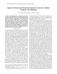
The global control scheme can be seen in Figure
2. The disturbance reference is a virtual input, representing
all plant mismatches referred to the system input.
The active state of the Kalman observer enables on-line estimation
of the disturbance, providing a feedforward compensation
action.
3. Experimental Setup
Experimental tests were done in a robotics testbed at the
DLR. The main components of this workstation are:
¯ A Manutec R2 industrial robot with a Cartesian position
interface running at Ñ×, with an input dead-time
of samples equivalent to ¼ Ñ×.
¯ A multi-processor host computer running UNIX, enabling
to compute the controller in each time step.
¯ A DLR lab end-effector which consists of a compliant
force/torque sensor providing force/torque measurements
every Ñ×. The technology data of the robot
and the stiffness of the DLR force sensor are summarized
in Table 3. The manipulator compliance is
lumped in the force sensor.
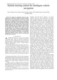
¯ Two cameras for stereo vision mounted on the endeffector
and a pneumatic gripper holding a steel peg of
¿¼ ÑÑ length. The peg is used to exert forces on the
top and side of a heavy steel block. The environment
is very stiff (Ã × Ã Û ). The vision cameras and the
pose sense are used for data fusion in a skill transfer
system [13]. A picture of the experimental setup is
depicted in Figure 3.
3. 1 Simulation Results
In this section some simulation results for the Ý force
component are presented. The goal of these simulations is
to observe the Ý force data for a step input. The contact
c­2000 Cyber Scientific Machine Intelligence & Robotic Control, 2(2), 19–27 (2000)

Force
Reference
Ä ½
È
· ·
Velocity
Reference
System Noise
Statistics
Measurement
Noise Statistics
Virtual
Disturbance
Reference
Ä ½
·
È
·
D
A
Velocity
Plant
à ×
×´½·Ì Ô×µ ×Ì Force
A
D
KALMAN
ACTIVE
OBSERVER
h
Pole Placement
Ä Ü
h
State Estimation
´Üµ
Disturbance Estimation (Active State)
Fig. 2
Global Control Scheme for each force dimension.
object is a heavy steel block. The end-effector is initially in
free space. A damping factor Ò ½was put in the design
guaranteeing the quickest response without overshoot. The
system time constant was chosen to be ½¼ Ì Ô where
Ì Ô ¼¼¿¾ × is the plant time constant (see Equation (3)),
and the nominal stiffness Ã × ¿ ÆÑÑ for the Ý direction.
It should be pointed out that can be specified to
have another value, enabling the system to have a faster or
slower response. The control algorithm and the dynamic
behaviour of the output force remain the same. The fastest
response is only limited by the maximum input velocity
that the robot can handle.
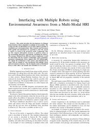
During the first seconds no desired force is given. The
robot is not moving ( ¼ Æ). Then, a desired force
of Ý ½¼ Æ is applied. The end-effector starts to move
along the Ý direction with a constant velocity till it reaches
contact. The contact appears at seconds. After contact,
the force response should have the desired second-order
behaviour. Finally a desired force of Æ is put at ½
seconds. Figure 4 shows the results for underestimated (a)
and overestimated (b) stiffness. Equations (5) establish the
relation between the design parameter ½ and the model
stiffness Ã × . It can be inferred that underestimated stiffness
originates a step response with undershoot, and overestimated
stiffness a step with overshoot.
Fig. 3
Experimental Setup
3. 2 Experimental Results
In the first experiment (Figure 5.a) the design stiffness
was considered as Ã × ¾, i.e., ½´Öе
½¾ ½´ÑÓе. In the second experiment (Figure 5.b)
Ã × ¿¼. Hence, theoretically there is a match (see Table
3) between the designed and real ½ parameter. The
simulation results of Section 3. 1 are consistent with the
experimental results. A detailed look of the force curve for
the matched situation reveals that the curve suffers from
the same pathology as the one obtained in the first experiment.
The real Ã × stiffness for the Ý direction is a bit
bigger than the nominal value referred in Table 3. Experiments
with this force control setup can be used to obtain
better values for the stiffness.
4. Noise-Based Switch Control
An important topic related with force control is the analysis
of the contact transition for a manipulator with a contact
sensor [15]. Generally, when establishing contact, the
manipulator and the target object have different velocities.
Thus, despite the force feedback, a force overshoot
in the transient process is unavoidable, and may be high.
To accomplish robustness between contact and non-contact
states, a noise-based control strategy was followed. If the
signal to noise ratio at the plant output ´ËÆ µ «, where
« is an acceptable threshold, it is assumed that the robot
is in free space for that dimension. In this case, it makes
no sense to perform any force control. The state feedback
is switched off, that is, the system is running in open loop.
The transfer function is given by Equation (3). A constant
velocity is reached for a step reference. It should be highlighted
that the cruise velocity is function of the expected
stiffness for the free-contact direction. In Figure 6, Ä ½ has
a key role in the approach phase. The bigger the stiffness
is for one force dimension, the smaller Ä ½ is, giving a robust
velocity approach before contact. Once in contact, the
state feedback is switched on, and Ä ½ prevents steady state
error to a step input. In the simulations as well as in the
experiments « ¾. Hence, a signal to noise ratio less than
c­2000 Cyber Scientific Machine Intelligence & Robotic Control, 2(2), 19–27 (2000)

2
½ ½¿ ½
2
½ ¾
0
Reference
0
Reference
-2
-2
Newton
-4
Newton
-4
-6
-6
-8
-8
-10
-10
-12
0 5 10 15 20
time (s)
-12
0 5 10 15 20
time (s)
(a)
(a)
2
½ ½ ½¿
2
½ ¿¼
0
Reference
0
Reference
-2
-2
Newton
-4
Newton
-4
-6
-6
-8
-8
-10
-10
-12
0 5 10 15 20
Fig. 4
time (s)
(b)
Simulation results for (a) underestimated stiffness, ½´Öе
½¿ ½´ÑÓе, and (b) overestimated stiffness ½´Öе
½´ÑÓе½¿.
¾ means that the end-effector is in free space.
5. Skill Transfer System
The force controller was applied for all 6 DOF in a skill
transfer system to perform the peg-in-hole task. Figure 6
gives an overview of the skill transfer system. The main
goal is the Human-Robot skill transfer of the peg-in-hole
task [13]. The task was previously performed by a human
where the forces, torques and velocities of the peg were
recorded function of its pose. The robot should be able
to perform the same task in a robust way after the skill
transfer. The force module is an important part of the system,
since it tries to output the desired force/velocity to
the peg, given a certain geometric information (pose and
vision data). This force controller can easily handle two
reference inputs (force), and Ú (velocity). The natural
constraints imply complementarity of the reference signals,
i.e., when is different than zero, Ú is almost zero, and
vice-versa. When Ú it means that the robot is in free
space. Thus, its behaviour is to follow the reference velocity
(open loop control), as was already explained. On the
contrary, when Ú the robot is in contact. The sum
of the reference signals corresponds in this case to a natural
switch between force and velocity control. Composing
-12
0 5 10 15 20
Fig. 5
time (s)
(b)
Experimental data of the force controller with: (a) underestimated
stiffness, Ã × ¾ and (b) nominal matching, Ã × ¿¼. These
data were obtained directly from the force sensor without any filtering.
The filtering and estimation is done in the Kalman Active
Observer.
velocity and force references can be seen in [3].
6. Conclusions
A systematic procedure was developed to design an explicit
force controller for manipulators with arbitrary deadtime.
The discrete closed loop system has always a secondorder
behaviour defined by the the desired damping factor
and natural frequency Û Ò . Guidelines to quantify the
Kalman matrices were referred. The introduction of an
active state enables the separation between truncation errors
and unknown errors in a natural way. Hence, the noise
analysis can be decoupled and easily handled. The active
state is a random variable that ”tracks” the disturbances due
to mismatches between real and model plants, providing a
global feedforward compensation action. Simulation results
showed good performance of the force controller for
the Ý dimension. The controller was successfully tested in
a Skill Transfer System at the DLR.
References
[1] K. J. Åström and B. Wittenmark. Computer Controlled Systems:
Theory and Design. Prentice Hall, 1997.
[2] S. M. Bosic. Digital and Kalman Filtering. Edward Arnold, 1979.
c­2000 Cyber Scientific Machine Intelligence & Robotic Control, 2(2), 19–27 (2000)

Skill Transfer
Module
Ú
Vision 1
ANN
Ó
Ú Ó
Fusion
Module
Ú
Ú
ANN
ANN
Vision 2
Pose
Desired
Compliant
Motion
·
È
Robot
Ü
DLR
Force Sensor
·
Ä ½
State Feedback
Kalman
Active
Observer
Ó
Ú Ó
Force/Velocity Controller
Fig. 6
Skill Transfer System giving emphasis in the Force/Velocity Controller.
[3] S. Chiaverini and L. Sciavicco. The parallel approach to
force/position control of robotic manipulators. In IEEE Trans. on
Robotics and Automation, volume 9, pages 361–373, 1993.
[4] R. Cortesão and R. Koeppe. Sensor fusion for human-robot skill
transfer systems. In RSJ Int. J. on Advanced Robotics. Special Issue
on ”Selected Papers From IROS’99”, October 2000. (to appear).
[5] R. Cortesão, R. Koeppe, U. Nunes, and G. Hirzinger. Explicit force
control for manipulators with active observers. In IEEE Int. Conf.
on Intelligent Robots and Systems, (IROS’2000), Japan, 2000. (to
appear).
[6] R. Cortesão, F. Millela, and U. Nunes. Joints robust position control
using linear kalman filters. In Int. Workshop on Advanced Motion
Control (AMC’98), pages 417–422, Portugal, 1998.
[7] K. Fujiyama, M. Tomizuka, and R. Katayama. Digital tracking controller
design for cd player using disturbance observer. In Int. Workshop
on Advanced Motion Control (AMC’98), pages 598–603, Portugal,
1998.
[8] A. C. Gelb. Applied Optimal Estimation. The MIT Press, 1973.
[9] D. Gorinevsky, A. Formalsky, and A. Schneider. Force Control of
Robotic Systems. CRC Press, 1997.
[10] G. Hirzinger. Robot-teaching via force-torque-sensors. In Proc. of
the Sixth European Meeting on Cybernetics and Systems Research,
1982.
[11] G. Hirzinger. Sensory feedback in robotics state-of-the-art in research
and industry. In Preprints of the 10th World IFAC Congress
on Automatic Control, volume 4, pages 204–210, 1987.
[12] A. Jazwinski. Stochastic Processes and Filtering Theory. Academic
Press, 1970.
[13] R. Koeppe and G. Hirzinger. Sensorimotor compliant motion from
geometric perception. In Proc. of the IEEE Int. Conf. on Intelligent
Robots and Systems, (IROS’99), volume 2, pages 805–811, Korea,
1999.
[14] P. Maybeck. Stochastic Models, Estimation, and Control, volume 1.
Academic Press, 1979.
[15] J. Mills and D. Lokhorst. Stability and control of robotic manipulators
during contact/noncontact task transition. In IEEE Trans. on
Robotics and Automation, volume 9, pages 148–163, 1993.
[16] C. Natale, R. Koeppe, and G. Hirzinger. A systematic design procedure
of force controllers for industrial robots. In IEEE Trans. on
Mechatronics, June 2000. (to appear).
[17] Y. Oh, W. K. Chung, and I. H. Suh. Disturbance observer based
robust impedance control of redundant manipulators. In Proc. of
the IEEE Int. Conf. on Intelligent Robots and Systems, (IROS’99),
volume 2, pages 647–652, Korea, 1999.
[18] H. Sorenson. Kalman filtering techniques. In Advances in Control
Systems. Academic Press, 1966.
[19] S. Yoshikawa. Foundations of Robotics: Analysis and Control. MIT
Press, 1990.
Biographies
Rui Cortesão was born in Coimbra, Portugal, in 1971. He received
the B.Sc. degree in Electrical Engineering, and the M.Sc.
degree in Systems and Automation from the University of Coimbra
in 1994 and 1997 respectively. He is currently pursuing the
Ph.D. degree in Electrical Engineering at the University of Coimbra,
with the DLR (German Aerospace Center) collaboration. He
joined the Electrical Engineering Department of the University
of Coimbra in 1998, where he is currently a Teaching Assistant.
He is a researcher of the Institute of Systems and Robotics (ISR).
His research interests include data fusion, control, fuzzy systems,
neural networks, and in general, intelligent architectures applied
to robots.
Ralf Koeppe received the ”Master of Science” degree in Mechanical
Engineering from Portland State University, Oregon in
1989, and the ”Diplom-Ingenieur” in Mechanical Engineering
c­2000 Cyber Scientific Machine Intelligence & Robotic Control, 2(2), 19–27 (2000)

form University of Stuttgart, Germany in 1992. Since 1992 he is
with the DLR (German Aerospace Center) Institute of Robotics
and Mechatronics, Germany. He has been leading research
projects in Neuro-Control since 1994, and directing research in
High-Fidelity Telepresence and Teleaction within the DFG Collaborative
Research Center (SFB) 453 since 1999. In 1996 he
was visiting researcher at Yoshikawa’s Robot Laboratory at Kyoto
University, Japan. He is currently completing his Ph.D. in
Mechanical Engineering as an external candidate of the Institute
of Robotics at ETH Zürich in Switzerland with the dissertation
‘Sensorimotor Skill Transfer of Compliant Motion’.
Urbano Nunes received the B.Sc. and Ph.D. degrees both in
Electrical Engineering from the University of Coimbra, in 1983
and 1995, respectively. He joined the Electrical Engineering Department
of the University of Coimbra in 1983, where he is currently
an Assistant Professor. He is a researcher of the Institute
of Systems and Robotics (ISR), where in the Coimbra site
is the coordinator of the Intelligent Control & Robotics Laboratory
(IC&R). He is a member of the editorial board of the Journal
on Machine Intelligence & Robotic Control, and a member of the
IFAC Technical Committee TC/MIL on Low Cost Automation
(1999 to 2002), IEEE, SIRES, and AAATE. His research interests
include control theory & application, intelligent control, robotics,
human-oriented robotics, and industrial automation.
Gerd Hirzinger received the ”Dipl.-Ing.” degree and the doctor’s
degree from the Technical University of Munich, in 1969
and 1974, respectively. In 1969 he joined DLR (the German
Aerospace Center) where he first worked on fast digital control
systems. In 1976 he became head of the automation and robotics
laboratory of the DLR. Since 1991 he has been Director of the
DLR Institute of Robotics and Mechatronics. He is IEEE fellow,
vice program chairman of the IEEE Conference on Robotics
and Automation 1994, and program chairman of IROS (Intelligent
Robot Systems Conference) 1994. For more than seven years
he has been chairman of the German Council on Robot Control.
c­2000 Cyber Scientific Machine Intelligence & Robotic Control, 2(2), 19–27 (2000)