Reactive Local Navigation - ISR-Coimbra

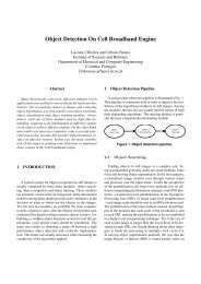
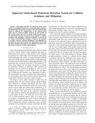
obstacle on the curvature defined by the velocity (v, ),measured by r.γ , where r = v ω is the radius of the circulartrajectory and γ the angle between the intersection with theobstacle and robot position. The accelerations for breakageare v& b and ω&b .Introducing a rectangular dynamic window, we couldreduce the search space to all velocities that can be reachedwithin the next time interval, according to the dynamiclimitations of the robot, given its current velocity and itsacceleration capabilities. The dynamic window Vd is definedas,{( v, ω ),v∈[ −v& . h,+ vh &.] ∧ ω ∈[ ω − & ω.h,ω + & ω h]}Vd = v c v cc c . (2)where h is the time interval during which accelerations v& andω& will be applied and ( , )v ω is the current velocity.ccTo determine the next motion command all admissiblevelocities within the dynamic window are considered,forming the resulting search space Vr defined asVr= Vs∩Va∩Vd. Among those a velocity is chosen thatmaximise a certain objective function (linear combination ofthree functions) where the alignment of the robot to a goalposition, the distance to the closest obstacles and its velocitycould be considered, as in the following expression:( , ω ) ( α ( , ω ) β ( , ω ) δ ( , ω ))G v = Max head v + dist v + vel v (3)The function ( v, ω) = 1 − θ πhead , where is the anglebetween the direction of motion and the goal heading, ismaximal to trajectories that are directed towards the goalposition. For a realistic measure of the target heading wehave to consider the dynamics of the rotation, therefore iscomputed at the predicted position that the robot will reachwhen exerting maximal deceleration after the next interval.vel v,ω is used to evaluate the progress of theThe function ( )robot on its trajectory. The three components of the objectivefunction are normalized to the interval [0,1].Parameters α, β and δ are used to weight the differentcomponents. Their values are crucial to the performance ofthe method and robot behaviour.Using this approach, robust obstacle avoidance behaviorshave been demonstrated at high velocities [9]. However,since the dynamic window approach only considers goalheading and no connectivity information about free space, itis still susceptible to local minima. Figures 1a) and 1b) showsa robot scan with a moving object and the respective velocityspace, with a dynamic window for v& =50cm/s 2 andω& =60º/s 2 .IV. VELOCITY OBSTACLE APPROACHThe VO approach [8] creates a velocity space, where setsof object avoiding velocities and object colliding velocitiesare computed. Avoidance manoeuvres could be done byselecting velocities to avoid a future collision within a giventime-horizon, considering the dynamic constraints of therobot.To compute the VO, we consider two circular objects, Aand B, at time t 0, with velocities v andA v . Let the circle ABrepresents the mobile robot and the circle B represents theobstacle. First, we reduce the mobile robot to a single point and enlarge the object circle B with the radius of A,creating Bˆ (see Fig.2). Position and velocity vectors areattached to its centres. Then the Collision Cone CC , set ofA,Bcolliding relative velocities between  and Bˆ , is defined by{ | λ ˆ 0}CC = v ∩ B ≠ (4)A, B A, B A,Bwhere vA,Bis the relative velocity of  with respect to Bˆ ,vA,B= vA − v , andBλA,Bis the line of v . This cone is theA,Bgray sector with apex in  , bounded by two tangents λ andfλrfrom  to Bˆ . Any relative velocity that lies inside theCC will cause a collision between A and B. The VO isA,Bobtained byVO = CC ⊕ v(5)A,BBλ A,BBˆλ fv Bλ rCC A,B VO BRAVRv A,BXYSv AÂUWZTa) b)Fig. 1. (a) Robot workspace simulation. (b) Velocity space-Vs. Thegray area represents the non-admissible velocity tuples. Therectangle represents the dynamic window-Vd. Four different pointsare represented in both Figures with the same number.v BFig. 2. Schematic representing two colliding objects, the mobilerobot A, circle (--), and the obstacle B, circle (-.-). The circle (⎯)represents the object B enlarged with the radius of A. The velocityobstacle (VO) and the reachable avoidance velocity (RAV) areas,which represent sets of relative velocities, are shown in gray.

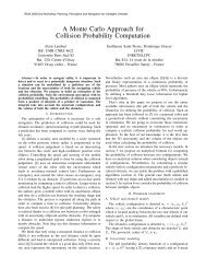
where ⊕ is the Minskowski vector sum operation, whichadds the velocity v to each velocity inBCC . To avoidA,Bmultiple obstacles, the union of individual velocity obstaclesmis done by VO = ∪i=1VOwhere m is the number of obstacles.BiThe next step is the computation of the set of velocitiesthat are dynamically reachable by the robot in the next timeinterval. The reachable velocities (RV) set is schematicallyrepresented in Fig. 2 by the polygon RSTU. The set ofreachable avoidance velocities (RAV), is defined as thedifference between the RV and the VO, polygons YSTZ andRXWU. A manoeuvre of avoiding obstacle B can becomputed by selecting any velocity in RAV, for examplewith an objective function like (3).It is also possible to choose different types of avoidancemanoeuvres, by selecting on which side of the obstacle themobile robot will pass. Velocities in RAV sub-set YSTZ willgive to the robot the possibility to avoid the obstacle from therear, and the sub-set RXWU will allow a front side avoidancemanoeuvre.V. LRF BASED OBSTACLE DETECTIONOur object detection system [4] is laser range finder basedand composed by four procedures: the segmentation, theclassification, the tracking and the collision detection (seeFig. 3). Object detection is achieved by the segmentation ofone or two consecutive scan sets, and vectorization of thesegments found. Object tracking is also possible from theobject classification procedure presented in this paper.Finally a collision detection procedure estimate futurecollisions between the robot and the objects detected.Localization Data(x,y,θ,goal)One Data SetLocal MapGrid BasedLaserOne/Two Data SetsStatic ObjectsSegmentationDynamic ObjectsOur object detection method is quite similar to theDietmayer et al. [6] method. Some modifications wereintroduced in the data preparation before the segmentation,and in the segments filtration process [4].In this work the LRF has a scan angle of 180°, with anangular resolution ∆α. The laser range data measured in theinstant k is represented by the set LRF K , of N data points P i ,with angle α i and distance value r i .A. Segmentation⎧⎪⎛αi⎞ ⎫⎪LRFk= ⎨Pi= ⎜ ⎟, i ∈[ 0, N ] ⎬⎪⎩⎝ ri⎠ ⎪⎭The segmentation process is based in the computation ofthe distance between two consecutive scan points (see Fig.4),calculated by( )2 2i i+ 1 i+ 1 i i+ 1 i i+1 i(6)d P, P = P − P = r + r −2r r cos ∆ α (7)If the distance is less than the threshold chosenwith( , ) min { , }d P P ≤ C + C r r (8)i i+ 1 0 1 i i+1( α )C1 = 2 1− cos ∆ (9)the point P i+1 belongs to the same segment as point P i . Theconstant C 0 allows an adjustment of the algorithm to noiseand strong overlapping of pulses in close range [6]. Theconstant C 1 is the distance between consecutive points ineach scan. This distance is also used to search the scan data,on the left and on the right, for points not selected in the dataanalysis. This operation gives the possibility to the algorithmto catch points with different dynamic activity from the restof the points just selected, like edge segment corners.Special tests could be done to combine segments thatprobably belong to the same object.Segments have a minimum size established in thebeginning (3 points) though pairs and isolated scan points arerejected. This is a very simple way of noise filtering.Velocity Space ApproachHeading Velocity DistanceClassificationTrackingCollision DetectionSEG2α β δMax(Σ)ε = 1 , If collision is detected;ε = 0 , otherwise.SEG4SEG3SEG1P i+1r i+P i∆αr i(v,ω)Fig. 3 . Laser range finder based obstacle detection system.Fig. 4. Schematic representing the segmentation processapplied to a hypothetical scan data.

B. Object ClassificationAfter the basic segmentation process, the segments foundedneed to be described by a set of points {A,B,C}, where {A} isthe closest point to the sensor and the other two {B,C}, thetwo segment extremes. Object classification could be donewith a certain probability, by matching the segmentrepresentation data, points {A,B,C}, with models of possibleobjects that could exist in the robot scene. Generally, mostobjects of interest in the robot’s or vehicle environment areeither almost convex or can be decomposed into almostconvex objects. A database of such possible objects isnecessary, and a priori knowledge of the workingenvironment is crucial to create it.E. ExampleUsing a SICK LMS 200 indoor LRF with a scanningfrequency of 75Hz and an angular resolution of 0.5° for a180° scan, we show in Fig. 5, real comparing results betweenour two-scan object detection algorithm [4] and the one-scanobject detection approach [6], for a Scout robot moving with1m/s in front of another Scout equipped with a LRF. Fromthe two-scan algorithm results only data segments formoving objects, otherwise, the one-scan algorithm give us allthe objects found in the scan data.C. Object TrackingIn order to perceive the object motion it is necessary toselect a reference point of the object which could be thesegment centre or point A. Usually, segment point A is theone chosen [8, 6]. In this work the tracking system issimulated and considered as optimal. because our goals arethe validation of the scanning algorithms and the reactivenavigation approaches. A discrete Kalman Filter basedtracking system is under development.D. Collision DetectionThe collision detection process predicts inside a predeterminedtemporal window (n time intervals) if any of theobjects detected collide with the robot. This process is doneassuming that the following statement is true: ‘two linesegments do not intersect if their bounding boxes do notintersect’ [5]. The bounding box of a geometric figure is thesmallest rectangle that contains the figure and whosesegments are parallel to the x-axis and y-axis. The boundingbox of a line segment p1 p2is represented by the rectangleˆ , ˆpˆ = xˆ , yˆand upper right( p1 p2 ) with lower left point1 ( 1 1 )point pˆ 2= ( xˆ ˆ2,y2) , where xˆ 1min ( x1 , x2)yˆ = min ( y , y ) , xˆ = max ( x , x ) and yˆ max ( y , y )1 1 22 1 2= ,= .2 1 2Two rectangles, represented by lower left and upper rightˆ , ˆ pˆ, p ˆ , intersect if and only if thepoints ( p p ) and ( )1 23 4following conjunction is true,( xˆ xˆ ) ( xˆ xˆ ) ( yˆ yˆ ) ( yˆ yˆ)≥ ∧ ≥ ∧ ≥ ∧ ≥ (10)2 3 4 1 2 3 4 1In this work, the bounding boxes represent objects and theirpredicted trajectory. It is assumed that all known dynamicactivity are constant in the next n time samples (for example,with n=20 we can predict the collision of moving objectswith 1m/s in a range of 4 m, with h=0.2s). In Fig. 5b) it ispresented the bounding boxes associated to all detectedobjects. The bounding box associated to the moving object infront of the robot represents the object and its trajectory forthe next n time intervals.a) b)Fig. 5. (a) Representation of the two-scan object detectionalgorithm [4]; (b) Representation of the one-scanobject detection approach [6], with the boundingboxes used in the collision detection.VI. REACTIVE LOCAL NAVIGATION METHODOur method, combines a LRF based object detectionmethodology with a velocity based approach, like thedynamic window. Similar to Fiorini’s VO approach, we havea collision avoidance technique, which takes into account thedynamic constraints of the robot and the motion constraintsof the nearby objects. As shown in figures 6a) and 6b), forthe same situation, both approaches consider the dynamicconstraints of the robot, throughout the RAV area in Fig. 6a)and the Vr search space of DW area in Fig. 6b).This method aims to calculate avoidance trajectories simplyby selecting velocities outside a predicted collision cone,penalizing the cone and nearby velocity areas and adding abonus to escape velocities.a) b)Fig.6 .a) VO collision cones repesentation. The static obstaclescollision cones are in white and the dynamic obstaclecollision cone is in dark. b) DW representation of thebonus cone for the same situation in (a).

The new objective function to be maximised is:( , ) = ( α ( , ω ) + β ( , ω ) + δ ( , ω ) + ε ( , ω ))(11)G v w Max head v dist v vel v bonus vwhere the alignment of the robot to a goal position, thedistance to the closest obstacles and its velocity can becombined with a bonus/penalty function.Function ( , )bonus v ω is described as follows,⎧ ⎡vv ⎤⎪ w∈ ,1 , ⎢ − ∆ ω + ∆ωrˆrˆ⎥− ⎣ ⎦⎪bonus( v, ω) = ⎨ 0 ,otherwise⎪ 1 ,⎪⎡ vv ⎤w∈ − − ∆ω,− + ∆ω⎪⎢ rˆ+ ∆ R rˆ+ ∆R⎥⎩ ⎣ ⎦(12)where rˆ is the estimated collision radius, ∆ ω an angularincrement necessary to penalise the collision area and nearbyareas. The value of ∆ ω depends on the robots dynamicconstraints and on collision detection information, such asthe proximity to obstacles and relative velocities between therobot and the obstacles. This prevents the robot to getundesirable collisions, from unknown changes in the objectpath. The parameter ∆ R is necessary to compensate thecollision radius rˆ when the radius value is too big.From the estimated robot position we calculate thetrajectory collision radius through some trigonometricequalities. Knowing the robot’s and object’s actualposition, P andRPO, and their actual velocities, it is easy tocompute their estimated positions, P and ˆR P (see Fig. 7).ˆOConsidering the inner triangles of the collision arc betweenthe robot and objects estimated positions, we have∆ABC~ ∆ DBC , and the following equalities are true,Consideringb BD BC c= = = ,a AB BD b2rˆ= a + c we obtain21 ⎛ b ⎞rˆ= ⎜ + a⎟2 ⎝ a ⎠2b= ac (13)(14)All the components of the objective function arenormalized to the interval [0,1]. Parameters α, β and δ areused to weight the different components.( x y )P O o, k , o,kPˆO( x y )o, k + 1,o,k + 1R ˆ( v,ω )bP ˆR ( xr, k + 1,yr,k + 1)cA a B C( x y )P R r, k , r,kFig. 7. Collision avoidance based on object motion prediction: P ,RP – actual robot / object position,OP , ˆR P - estimatedˆOrobot/object position, ˆR - estimated collision radius.narrow indoor real spaces, where the LRF is always detectingstatic objects, the building walls.Objects were modelled as rectangular shapes, for people orother robots moving in the corridor. The user in thebeginning of a new simulation could specify their movingdirection, velocity and diameter. In all examples the robotstarted without any knowledge of the environment.Several tests were done to compare the basic DW approach,our reactive navigation system and the VO approach. A greateffort was done to maintain similar as possible all simulationparameters. The optimization function used to select the bestvelocity in Vr and in RAV is equal to (3), with parametervalues {α=0.8, β=0.5, δ=0.2}. Some differences exist in thedist function settings, because one spans a (v,ω) space andthe other a Cartesian space.In Fig.8, we have an avoidance manoeuvre between twomoving objects. The robot starts with v 0 =50cm/s aligned withthe goal position. The robot must pass between to movingobjects because the object in front is moving in the goaldirection. All methods have a similar behaviour.D(v=50cm/s)VII. SIMULATION RESULTSExtensive simulation tests were done to validate and testthe methods exposed above. A sensor model was created forthe LRF with the following specifications: each scan has anangle of view of about 180°, the maximum distancemeasured between the target and the sensor was 300 cm, with±1 cm of accuracy. The sensor is centred with the robots coordinateaxis, aligned with the motion axis.The workspace is a typical indoor dynamic environment, acorridor with two escape ways for doors and a turn on thetop, see Fig.8. The workspace dimensions are similar to(1m/s)(v0=50cm/s)Fig. 8. Avoidance manoeuvre between two moving objects.

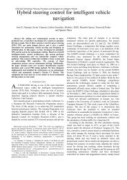
In Fig. 9a) one of the goals of this work is shown. We havea robot moving aligned with the goal position, but the objectin front is moving in the robots direction. The success of theavoidance manoeuvre is totally dependent on the relativevelocity value between the robot and the moving object. Thevelocity space of the basic DW approach represents onlystatic information, so this approach can not deal with thissituation. The concept of “select velocities that allow therobot to stop before it reaches a obstacle” is only true if thereare not any moving object in the search space. With the basicDW the robot tries to keep the heading orientation aspossible and some time later tries to avoid a moving objectthat it perceives as being static. The VO approach easily dealwith this situations because the collision cones impels therobot automatically in a secure avoidance trajectory. Ourreactive algorithm introduces in the velocity space a collisioncone similar to the VO approach, giving to the DW approachthe ability to deal with situations like this.In Fig. 9b) an abortive manoeuvre is shown. Both strategiestried to pass between the obstacles, and non of them havestopped without hitting the obstacles, or tried to follow theobject moving to the goal direction with slow velocity.VIII. CONCLUSIONSResults from both reactive navigation strategies shows thatboth approaches deal with success to unforeseen changes inthe environment or to unpredictable objects blocking theirtrajectories. Some of the advantages of the VO approach areconcerned to its space (v x ,v y ) representation, which has robotobstaclescollision information represented, giving to therobot the possibility to avoid obstacles as soon as they aredetected. The (v,ω) space only represents the robot’s velocitylimit to hit object in their sensory range limit.Our local navigation scheme looks promising, in the waythat it gives to the DW approach the possibility to avoidobstacles as soon as they are detected, too.(50cm/s)(v0=50cm/s)(30cm/s)a) b)(30cm/s)(v0=50cm/s)Fig. 9 a) Avoidance manoeuvre for a robot moving aligned with thegoal, with an object moving in the robots direction.b) Abortive manoeuvre.Future work will be done in local space representation(topological and geometric). A perception scheme that givesto the robot all local knowledg necessary to navigate betweenmultiple moving object, negotiating secure trajectories, isnecessary.IX. ACKNOWLEDGEMENTSThis work was partially supported by a PhD student grant(BD/1104/2000) given to the author Daniel Castro by FCT(Fundação para a Ciência e Tecnologia).X. REFERENCES[1] K.Arras, J.Persson, N.Tomatis and R.Siegwart, ”Real-TimeObstacle Avoidance for Polygonal Robots with a ReducedDynamic Window”, in IEEE Int. Conf. on Robotics andAutomation ICRA’02, Washington DC, May 2002, pp.3050-3055.[2] J. Borenstein and Y. Koren, “The Vector Field Histogram –Fast Obstacle Avoidance for Mobile Robots”, IEEE Trans. onRobotics and Automation, 7(3), June 1991, pp. 278-288.[3] O. Brock and O. Khatib, “High-Speed Navigation Using theGlobal Window Approach”, in IEEE Int. Conf. on Roboticsand Automation ICRA’99, Detroid, May 1999, pp.341-346.[4] D. Castro, U. Nunes and A. Ruano, ”Obstacle Avoidance inLocal Navigation”, in IEEE Mediterranean Conference onControl and Automation MED 2002, Lisbon, July 2002.[5] T. Cormen, C. Leiserson and R. Rivest, Introduction toAlgorithms, The MIT Press, 1999.[6] K. Dietmayer, J. Sparbert and D. Streller, “Model BasedObject Classification and Tracking in Traffic Scenes fromRange Images”, in IEEE Intelligent Vehicle Symposium -IV2001, Tokyo, May 2001.[7] W. Feiten, R. Bauer and G. Lawitzky, “Robust ObstacleAvoidance in Unknown and Cramped Environments”, in IEEEInt. Conf. on Robotics and Automation ICRA’94, San-Diego,May 1994, pp.2412-2417.[8] P. Fiorini and Z. Shiller, “Motion Planning in DynamicEnvironments using Velocity Obstacles”, Int. Journal onRobotics Research, 17 (7), 1998, pp.711-727.[9] D. Fox, W. Burgard. and S. Thrun, “The Dynamic WindowApproach to Collision Avoidance”, IEEE Robotics andAutomation Magazine, 4(1), March 1997, pp. 23-33.[10] D. Fox, W. Burgard., S. Thrun and A. Cremers, “A HybridCollision Avoidance Method for Mobile Robots”, in IEEE Int.Conf. on Robotics and Automation ICRA’98, 1998, pp.1238-1243.[11] H. Hu and M. Brady, “A Bayesian Approach to Real-timeObstacle Avoidance for Mobile Robots”, Autonomous Robots,1, 1994, pp. 69-92.[12] M. Khatib and R. Chatila, “An Extended Potential FieldApproach for Mobile Robot Sensor-based Motions”, in IEEEInt. Conf. on Intelligent Autonomous Systems - IAS’4, pp.490-496, 1995.[13] O. Khatib, “Real-time Obstacle Avoidance for Manipulatorsand Mobile Robots”, The Int. Journal of Robotics Research,5(1), pp.90-98, 1986.[14] J-C. Latombe, Robot Motion Planning, Kluwer AcademicPublishers, Boston, 1991.[15] R. Simmons, “The Curvature-Velocity Method for LocalObstacle Avoidance”, in IEEE Int. Conf. on Robotics andAutomation ICRA’96, Minneapolis, April 1996, pp.2275-2282.