Channel Coding I Exercises â WS 2012/2013 â - Universität Bremen
Channel Coding I Exercises â WS 2012/2013 â - Universität Bremen
Channel Coding I Exercises â WS 2012/2013 â - Universität Bremen

Create successful ePaper yourself
Turn your PDF publications into a flip-book with our unique Google optimized e-Paper software.
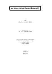
<strong>Channel</strong> <strong>Coding</strong> I<br />
<strong>Exercises</strong><br />
– <strong>WS</strong> <strong>2012</strong>/<strong>2013</strong> –<br />
Lecturer: Dirk Wübben, Carsten Bockelmann<br />
Tutor: Matthias Woltering<br />
NW1, Room N 2400, Tel.: 0421/218-62392<br />
E-mail: {wuebben, bockelmann, woltering}@ant.uni-bremen.de<br />
Universität <strong>Bremen</strong>, FB1<br />
Institut für Telekommunikation und Hochfrequenztechnik<br />
Arbeitsbereich Nachrichtentechnik<br />
Prof. Dr.-Ing. A. Dekorsy<br />
Postfach 33 04 40<br />
D–28334 <strong>Bremen</strong><br />
WWW-Server: http://www.ant.uni-bremen.de<br />
Version from November 7, <strong>2012</strong>
November 7, <strong>2012</strong><br />
I<br />
<strong>Exercises</strong><br />
1 Introduction 1<br />
Exercise 1.1: Design of a discrete channel . . . . . . . . . . . . . . . . . . . . . . . . 1<br />
Exercise 1.2: Statistics of the discrete channel . . . . . . . . . . . . . . . . . . . . . . 1<br />
Exercise 1.3: Binary symmetric channel (BSC) . . . . . . . . . . . . . . . . . . . . . 1<br />
Exercise 1.4: Serial concatenation of two BSC . . . . . . . . . . . . . . . . . . . . . . 1<br />
Exercise 1.5: Transmission of a coded data over BSCs . . . . . . . . . . . . . . . . . . 2<br />
2 Information theory 3<br />
Exercise 2.1: Entropy . . . . . . . . . . . . . . . . . . . . . . . . . . . . . . . . . . . 3<br />
Exercise 2.2: <strong>Channel</strong> capacity of a discrete memory-free channel . . . . . . . . . . . 3<br />
Exercise 2.3: <strong>Channel</strong> capacity of a BSC . . . . . . . . . . . . . . . . . . . . . . . . . 3<br />
Exercise 2.4: <strong>Channel</strong> capacity of the AWGN . . . . . . . . . . . . . . . . . . . . . . 4<br />
3 Linear block codes 5<br />
3.2 Finite field algebra . . . . . . . . . . . . . . . . . . . . . . . . . . . . . . . . . . . . . 5<br />
Exercise 3.1: 2-out-of-5-code . . . . . . . . . . . . . . . . . . . . . . . . . . . . . . . 5<br />
Exercise 3.2: Field . . . . . . . . . . . . . . . . . . . . . . . . . . . . . . . . . . . . 5<br />
3.3 Distance properties of block codes . . . . . . . . . . . . . . . . . . . . . . . . . . . . . 5<br />
Exercise 3.3: Error correction . . . . . . . . . . . . . . . . . . . . . . . . . . . . . . . 5<br />
Exercise 3.4: Sphere-packing bound . . . . . . . . . . . . . . . . . . . . . . . . . . . 6<br />
3.5 Matrix description of block codes . . . . . . . . . . . . . . . . . . . . . . . . . . . . . 6<br />
Exercise 3.5: Generator and parity check matrices . . . . . . . . . . . . . . . . . . . . 6<br />
Exercise 3.6: Expansion, shortening, and puncturing of codes . . . . . . . . . . . . . . 6<br />
Exercise 3.7: Coset decomposition and syndrome decoding . . . . . . . . . . . . . . . 7<br />
Exercise 3.8: <strong>Coding</strong> program . . . . . . . . . . . . . . . . . . . . . . . . . . . . . . 7<br />
3.6 Cyclic Codes . . . . . . . . . . . . . . . . . . . . . . . . . . . . . . . . . . . . . . . . 7<br />
Exercise 3.9: Polynomial multiplication . . . . . . . . . . . . . . . . . . . . . . . . . 7<br />
Exercise 3.10: Polynomial division . . . . . . . . . . . . . . . . . . . . . . . . . . . . 8<br />
Exercise 3.11: Generator polynomial . . . . . . . . . . . . . . . . . . . . . . . . . . . 8<br />
Exercise 3.12: Syndrome . . . . . . . . . . . . . . . . . . . . . . . . . . . . . . . . . 8<br />
Exercise 3.13: Primitive polynomials . . . . . . . . . . . . . . . . . . . . . . . . . . . 9<br />
Exercise 3.14: CRC codes . . . . . . . . . . . . . . . . . . . . . . . . . . . . . . . . 9<br />
3.7 Reed-Solomon- and BCH-codes . . . . . . . . . . . . . . . . . . . . . . . . . . . . . . 9<br />
Exercise 3.15: Reed-Solomon-codes . . . . . . . . . . . . . . . . . . . . . . . . . . . 9
November 7, <strong>2012</strong><br />
II<br />
Exercise 3.16: BCH-codes . . . . . . . . . . . . . . . . . . . . . . . . . . . . . . . . 9<br />
Exercise 3.17: Bit- and word error curves of BCH-codes . . . . . . . . . . . . . . . . 10<br />
4 Convolution codes 11<br />
4.1 Fundamental principles . . . . . . . . . . . . . . . . . . . . . . . . . . . . . . . . . . . 11<br />
Exercise 4.1: Convolution code . . . . . . . . . . . . . . . . . . . . . . . . . . . . . . 11<br />
4.2 Characterization of convolution codes . . . . . . . . . . . . . . . . . . . . . . . . . . . 11<br />
Exercise 4.2: Catastrophic codes . . . . . . . . . . . . . . . . . . . . . . . . . . . . . 11<br />
4.3 Distance properties of convolution codes . . . . . . . . . . . . . . . . . . . . . . . . . . 11<br />
Exercise 4.3: Distance properties of convolution codes . . . . . . . . . . . . . . . . . 11<br />
Exercise 4.4: Comparison of NSC- and RSC-codes . . . . . . . . . . . . . . . . . . . 11<br />
4.4 Puncturing of convolution codes of the rate 1/n . . . . . . . . . . . . . . . . . . . . . . 12<br />
Exercise 4.5: Puncturing of convolution codes* . . . . . . . . . . . . . . . . . . . . . 12<br />
4.5 Optimal decoding with Viterbi-algorithm . . . . . . . . . . . . . . . . . . . . . . . . . 13<br />
Exercise 4.6: Viterbi-decoding . . . . . . . . . . . . . . . . . . . . . . . . . . . . . . 13<br />
Exercise 4.7: Viterbi-decoding with puncturing . . . . . . . . . . . . . . . . . . . . . 13<br />
Exercise 4.8: <strong>Coding</strong> and decoding of a RSC code . . . . . . . . . . . . . . . . . . . . 13<br />
Exercise 4.9: Investigation to Viterbi-decoding . . . . . . . . . . . . . . . . . . . . . . 14<br />
Exercise 4.10: Simulation of a convolution-coder and -decoder . . . . . . . . . . . . . 14
November 7, <strong>2012</strong><br />
III<br />
General Information<br />
• The dates for the exercises are arranged in the lectures and take place in room N 2250 or N 2410.<br />
The exercises cover the contents of past lectures and contain a theoretical part and a programming<br />
part, in general. The students are advised to repeat the corresponding chapters and to prepare the<br />
exercises for presenting them at the board.<br />
• All references to passages in the text (chapter- and equation numbers) refer to the script: V. Kühn,<br />
“Kanalcodierung I+II” in german language. References of equations in the form of (1.1) refer to<br />
the script, too, whereas equations in the form (1) refer to solutions of the exercises.<br />
• Although MATLAB is used in the exercises, no tutorial introduction can be given due to the limited<br />
time. A tutorial and further information can be found in<br />
– MATLAB Primer, 3rd edition, Kermit Sigmon<br />
– Practical Introduction to Matlab, Mark S. Gockenbach<br />
– NT Tips und Tricks für MATLAB, Arbeitsbereich Nachrichtentechnik, Universität <strong>Bremen</strong><br />
– Einführung in MATLAB von Peter Arbenz, ETH Zürich<br />
available on http://www.ant.uni-bremen.de/teaching/kc/exercises/.<br />
• PDF-files of the tasks, solutions and MATLAB codes are available on<br />
http://www.ant.uni-bremen.de/de/courses/cc1/.<br />
Within the university net the additional page<br />
http://www.ant.uni-bremen.de/de/courses/cc1/<br />
is available. Beside the tasks and solutions you will find additional information on this page, e.g the<br />
matlab primer, the original paper of C. E. Shannon A mathematical theory of communication,<br />
some scripts and a preliminary version of the book ”Error-Control <strong>Coding</strong>” of B. Friedrichs!
1 INTRODUCTION November 7, <strong>2012</strong> 1<br />
1 Introduction<br />
Exercise 1.1<br />
Design of a discrete channel<br />
a) Given is a transmitting alphabet consisting of the symbols −3, −1, +1, +3. They shall be<br />
transmitted over an AWGN-channel, which is real valued and has the variance σN 2 = 1. At the<br />
output of the channel a hard-decision takes place, i.e. the noisy values are again mapped to the<br />
4 symbols (A out = A in ), where the decision thresholds in each case lies in the middle of two<br />
symbols. Calculate the transition probabilities P(Y µ |X ν ) of the channel and represent them in a<br />
matrix.<br />
b) Check the correctness of the matrix by checking the sums of probabilities to one.<br />
c) Determine the joint probabilities P(X ν ,Y µ ) for equally probable transmitting symbols.<br />
d) Calculate the occurrence probabilities for the channel output symbols Y µ .<br />
e) Calculate the error probability P e (X ν ) for the transmitting symbols X ν and the mean overall error<br />
probability P e .<br />
Exercise 1.2<br />
Statistics of the discrete channel<br />
a) Given are the channels in figure 1. Complete the missing probabilities.<br />
<strong>Channel</strong> 1 <strong>Channel</strong> 2<br />
0.2 X 0<br />
0.7<br />
Y 0 0.3 0.2 X 0<br />
0.8<br />
Y 0<br />
Y 1<br />
Y 1<br />
0.08<br />
X 1 Y 2<br />
X 1<br />
Y 2<br />
0.8<br />
Fig. 1: Discrete channel models<br />
Exercise 1.3<br />
Binary symmetric channel (BSC)<br />
a) The word 0110100 is transmitted by a BSC with the error probability P e = 0.01. Specify the<br />
probability of receiving the word 0010101, wrongly.<br />
b) Determine the probability of m incorrectly received bits at the transmission of n bits.<br />
c) For a BSC with the error probability P e = 0.01, the probability of more than 2 errors at words of<br />
the length 31 shall be determined.<br />
Exercise 1.4<br />
Serial concatenation of two BSC
1 INTRODUCTION November 7, <strong>2012</strong> 2<br />
Two BSC-channels with P e,1 and P e,2 shall be connected in series. Determine the error probability of<br />
the new channel.<br />
Exercise 1.5<br />
Transmission of a coded data over BSCs<br />
Use Matlab to simulate the transmission of coded data over a Binary Symmetric <strong>Channel</strong> (BSC) with<br />
error probability P e = 0.1. Apply repetition coding of rate R c = 1/5 for error protection.
2 INFORMATION THEORY November 7, <strong>2012</strong> 3<br />
2 Information theory<br />
Exercise 2.1<br />
Entropy<br />
a) The average information content H(X ν ) of the signal X ν (also called partial entropy) shall be<br />
maximized. Determine the valueP(X ν ), for which the partial entropy reaches its maximum value<br />
and specify H(X ν ) max . Check the result with MATLAB by determining the partial entropy for<br />
P(X ν ) = 0 : 0.01 : 1 and plotting H(X ν ) over P(X ν ).<br />
b) The random vector (X 1 X 2 X 3 ) can exclusively carry the values (000), (001), (011), (101) and<br />
(111) each with a probability of 1/5.<br />
Determine the entropies:<br />
1. H(X 1 )<br />
2. H(X 2 )<br />
3. H(X 3 )<br />
4. H(X 1 ,X 2 )<br />
5. H(X 1 ,X 2 ,X 3 )<br />
6. H(X 2 |X 1 )<br />
7. H(X 2 |X 1 = 0)<br />
8. H(X 2 |X 1 = 1)<br />
9. H(X 3 |X 1 ,X 2 )<br />
Exercise 2.2<br />
<strong>Channel</strong> capacity of a discrete memory-free channel<br />
Determine the channel capacity for the following discrete memory-free channel on condition thatP(X ν ) =<br />
1/3 is valid.<br />
X<br />
1/2<br />
0<br />
1/3<br />
1/6<br />
Y 0<br />
1/6<br />
X 1<br />
1/2<br />
1/3<br />
Y 1<br />
1/3<br />
1/6<br />
X 2 Y<br />
1/2<br />
2<br />
Exercise 2.3<br />
<strong>Channel</strong> capacity of a BSC<br />
a) Derive the capacity for equally probable input symbols P(X 0 ) = P(X 1 ) = 0.5 in dependence on<br />
the error probability for a binary symmetric channel (BSC).<br />
b) Prepare a MATLAB program, which calculates the capacity of an unsymmetric binary channel for<br />
the input probabilities P(x) = 0 : 0.01 : 1. It shall be possible to set the error probabilities P e,x0<br />
and P e,x1 at the program start. (Attention: P(y) must be calculated!)
2 INFORMATION THEORY November 7, <strong>2012</strong> 4<br />
x0<br />
1-P e,x0<br />
y0<br />
P e,x0<br />
1-P ex1<br />
x1<br />
P e,x1<br />
y1<br />
c) Determine the channel capacity for several error probabilities P e at a fixed input probability P(x)<br />
within MATLAB. Plot C(P e ).<br />
Exercise 2.4<br />
<strong>Channel</strong> capacity of the AWGN<br />
Derive the channel capacity for a bandwidth limited Gaussian channel (σ 2 n = N 0 /2) with a normal<br />
distributed input (σ 2 x = E s ) according to eq. (2.28).
3 LINEAR BLOCK CODES November 7, <strong>2012</strong> 5<br />
3 Linear block codes<br />
3.2 Finite field algebra<br />
Exercise 3.1<br />
2-out-of-5-code<br />
a) Given is a simple 2-out-of-5-code of the lengthn=5 that is composed of any possible words with<br />
the weight w H (c) = 2. Specify the code C. Is it a linear code?<br />
b) Determine the distance properties of the code. What is to be considered?<br />
c) Calculate the probability P ue of the occurrence of an undetected error for the considered code at<br />
a binary symmetric channel. The transition probabilities of the BSC shall be in the range 10 −3 ≤<br />
P e ≤ 0.5. Represent P ue in dependence on P e graphically and depict also the error rate of the<br />
BSC in the chart.<br />
d) Check the result of c) by simulating a data transmission scheme in MATLAB and measuring the<br />
not detected errors for certain error probabilities P e of the BSC.<br />
Hint: Choose N code words by random and conduct a BPSK-modulation. Subsequently, the<br />
words are superposed with additive white, Gaussian distributed noise, where its power corresponds<br />
to the desired error probability P e = 0.5 · erfc( √ E s /N 0 ) of the BSC. After a hard-decision of<br />
the single bit, the MLD can be realized at the receiver by a correlation of the received word and<br />
all possible code words with subsequent determination of the maximum. Subsequently, the errors<br />
have to be counted.<br />
e) Calculate the error probability P w at soft-decision-ML-decoding for the AWGN-channel.<br />
f) Check the results of e) with the help of simulations in the range −2 dB ≤ E s /N 0 ≤ 6 dB.<br />
Compare the obtained error rates with the uncoded case.<br />
Hint: You can use the same transmission scheme as in item d). But this time, the hard-decision<br />
has to be conducted after the ML-decoding.<br />
Exercise 3.2<br />
Field<br />
Given are the sets M q := {0,1,...,q −1} and the two connections<br />
• addition modulo q<br />
• multiplication modulo q<br />
Calculate the connection tables for q = 2,3,4,5,6 and specify, from which q results a field.<br />
3.3 Distance properties of block codes<br />
Exercise 3.3<br />
Error correction<br />
Given is a(n,k) q block code with the minimal distance d min = 8.
3 LINEAR BLOCK CODES November 7, <strong>2012</strong> 6<br />
a) Determine the maximal number of correctable errors and the number of detectable errors at pure<br />
error detection.<br />
b) The code shall be used for the correction of 2 errors and for the simultaneous detection of 5 further<br />
errors. Demonstrate by illustration in the field of code words (cp. fig. 3.1), that this is possible.<br />
c) Demonstrate by illustration in the field of code words, how many possibilities of variation of a<br />
code word have to be taken into consideration at the transmission over a disturbed channel.<br />
Exercise 3.4<br />
Sphere-packing bound<br />
a) A linear (n,2) 2 -block code has the minimal Hamming distance d min = 5. Determine the minimal<br />
block length.<br />
b) A binary code C has the parameters n = 15,k = 7,d min = 5. Is the sphere packing bound<br />
fulfilled? What does the right side minus the left side of the sphere packing bound (cp. eq. (3.7))<br />
state?<br />
c) Can a binary code with the parameters n = 15,k = 7,d min = 7 exist?<br />
d) Check, if a binary code with the parameters n = 23,k = 12,d min = 7 can exist.<br />
e) A source-coder generates 16 symbols, that shall be coded binary with a correction capacity of 4 in<br />
the channel coder. How great does the code rate have to be in any case?<br />
3.5 Matrix description of block codes<br />
Exercise 3.5<br />
Generator and parity check matrices<br />
a) State the generator- as well as the parity check matrix for a (n,1,n) repetition code with n = 4.<br />
What parameters and properties does the dual code have?<br />
b) The columns of the parity check matrix of a Hamming code of degreerrepresent all dual numbers<br />
from 1 to 2 r −1. State a parity check matrix for r = 3 and calculate the corresponding generator<br />
matrix. Determine the parameters of the code and state the code rate.<br />
c) Analyze which connection is between the minimal distance of a code and the number of linear<br />
independent columns of the parity check matrix H by means of this example.<br />
Exercise 3.6<br />
Expansion, shortening, and puncturing of codes<br />
a) Given is the systematical (7,4,3)-Hamming code from exercise 3.5. Expand the code by an<br />
additional test digit such that it gets a minimum distance of d min = 4. State the generator matrix<br />
G E and the parity check matrix H E of the expanded (8,4,4)-code.<br />
Hint: Conduct the construction with the help of the systematic parity check matrix H S and note<br />
the result from 3.5c.
3 LINEAR BLOCK CODES November 7, <strong>2012</strong> 7<br />
b) Shortening a code means the decrease of the cardinality of the field of code words, i.e. information<br />
bits are cancelled. Shorten the Hamming code from above to the half of the code words and state<br />
the generator matrix G K and the parity check matrix H K for the systematic case. What minimal<br />
distance does the shortened code have?<br />
c) Puncturing a code means gating out code bits which serves for increasing the code rate. Puncture<br />
the Hamming code from above to the rate R c = 2/3. What minimal distance does the new code<br />
have?<br />
Exercise 3.7<br />
Coset decomposition and syndrome decoding<br />
a) State the number of syndromes of the (7,4,3)-Hamming code and compare it with the number of<br />
correctable error patterns.<br />
b) Make up a table for the systematic (7,4,3)-Hamming coder which contains all syndromes and the<br />
corresponding coset leaders.<br />
c) The wordy = (1101001) is found at the receiver. Which information worduwas sent with the<br />
greatest probability?<br />
d) The search for the position of the syndrome s inHcan be dropped by resorting the columns ofH.<br />
The decimal representation of s then can directly be used for the addressing of the coset leader.<br />
Give the corresponding parity check matrix ˜H.<br />
Exercise 3.8<br />
<strong>Coding</strong> program<br />
a) Write a MATLAB-programm which codes and again decodes a certain number of input data bits.<br />
Besides it shall be possible to insert errors before the decoding. The(7,4,3)-Hamming code with<br />
the generator matrix<br />
and the parity check matrix<br />
G =<br />
⎛<br />
⎜<br />
⎝<br />
⎛<br />
H = ⎝<br />
1 0 0 0 0 1 1<br />
0 1 0 0 1 0 1<br />
0 0 1 0 1 1 0<br />
0 0 0 1 1 1 1<br />
0 1 1 1 1 0 0<br />
1 0 1 1 0 1 0<br />
1 1 0 1 0 0 1<br />
⎞<br />
⎟<br />
⎠<br />
⎞<br />
⎠<br />
shall be used.<br />
b) Extend the MATLABprogram for taking up bit error curves in the range 0 : 20dB.<br />
3.6 Cyclic Codes<br />
Exercise 3.9<br />
Polynomial multiplication<br />
Given are the two polynomials f(D) = D 3 +D +1 and g(D) = D +1.
3 LINEAR BLOCK CODES November 7, <strong>2012</strong> 8<br />
a) Calculate f(D)·g(D). Check the result with MATLAB.<br />
b) Give the block diagram of a nonrecursive system for a sequential multiplication of both polynomials.<br />
c) Illustrate the stepwise calculation of the polynomial f(D) · g(D) in dependence on the symbol<br />
clock by means of a table.<br />
Exercise 3.10<br />
Polynomial division<br />
Given are the two polynomials f(D) = D 3 +D +1 and g(D) = D 2 +D +1.<br />
a) Calculate the division off(D) byg(D). Check the result with MATLAB.<br />
b) Give the block diagram of a recursive system for a sequential division of the polynomial f(D) by<br />
the polynomial g(D).<br />
c) Illustrate the stepwise calculation of the polynomial f(D) : g(D) in dependence on the symbol<br />
clock by means of a table.<br />
Exercise 3.11<br />
Generator polynomial<br />
Given is a cyclic (15,7) block code with the generator polynomial g(D) = D 8 +D 7 +D 6 +D 4 +1.<br />
a) Indicate that g(D) can be a generator polynomial of the code.<br />
b) Determine the code polynomial (code word) in systematical form for the message u(D) = D 4 +<br />
D +1.<br />
c) Is the polynomial y(D) = D 14 +D 5 +D +1 a code word?<br />
Exercise 3.12<br />
Syndrome<br />
The syndromes s 1 to s 8 of a 1-error-correcting cyclic code are given.<br />
s 1 = 1 0 1 0 0<br />
s 2 = 0 1 0 1 0<br />
s 3 = 0 0 1 0 1<br />
s 4 = 1 0 0 0 0<br />
s 5 = 0 1 0 0 0<br />
s 6 = 0 0 1 0 0<br />
s 7 = 0 0 0 1 0<br />
s 8 = 0 0 0 0 1<br />
a) Determine the parity check matrix H and the generator matrix G.<br />
b) State the number of test digits n−k and the number of information digits k.<br />
c) What is the generator polynomial g(D)?<br />
d) How many different code words can be built with the generator polynomial g(D)?
3 LINEAR BLOCK CODES November 7, <strong>2012</strong> 9<br />
e) The code wordy 1 = (01101011) is received. Has this code word been falsified on the channel?<br />
Can the right code word be determined? If yes, name the right code word.<br />
f) Now the code wordy 2 = (10110111) has been received. Has this code word been falsified on<br />
the channel? Can the right code word be determined? If yes, name the right code word.<br />
Exercise 3.13<br />
Primitive polynomials<br />
Given are the two irreducible polynomials g 1 (D) = D 4 +D+1 andg 2 (D) = D 4 +D 3 +D 2 +D+1.<br />
Which of these two polynomials is primitive?<br />
Exercise 3.14<br />
CRC codes<br />
a) Generate the generator polynomial for a CRC code of the length n = 15.<br />
b) Determine the generator matrix G and the parity check matrix H.<br />
c) Now the efficiency of the CRC code shall be examined by considering the perceptibility of all<br />
burst errors of the length 4 ≤ l e ≤ n. Only error patterns with the l e errors directly succeeding<br />
one another shall be taken into consideration. Give the relative frequency of the detected errors.<br />
3.7 Reed-Solomon- and BCH-codes<br />
Exercise 3.15<br />
Reed-Solomon-codes<br />
a) A RS-code in theGF(2 3 ) that can correctt = 1 error shall be generated. Determine the parameters<br />
k, n and R c and state the maximal length of a correctable error in bit.<br />
b) Give the generator polynomial g(D) of the Reed-Solomon-code. Use the commands rspoly<br />
resp. eq. (3.77).<br />
c) The message u = (110 010 111 000 001) shall be coded. At the subsequent transmission 3 bits<br />
shall be falsified. How does the position of the error affect on the decoding result?<br />
d) Now a t = 2 errors correcting code in the GF(8) shall be designed. Again determine the<br />
parameters k and R c and give g(D).<br />
e) The wordy = (000100001011110010111) is received. Determine the syndrome, the error digit<br />
polynomial, the position of the error digits and the amplitudes of the errors. Use the commands<br />
rssyndrom, rselp, rschien and rserramp. What was the transmitted message (correction<br />
with rscorrect )?<br />
Exercise 3.16<br />
BCH-codes<br />
a) We now want to design a t = 3 errors correcting BCH-code in the GF(2 4 ). Form the cyclotomic<br />
cosets K i with the command gfcosets. Which sets can be combined to one set K i for fulfilling<br />
the challenge t = 3. Which parameters does the resulting BCH-code have?
3 LINEAR BLOCK CODES November 7, <strong>2012</strong> 10<br />
b) With the command bchpoly all valid parameter combinations can be announced, at declaration<br />
of the parameters n and k bchgenpoly supplies a generator polynomial g 1 (D) and the polynomialsm<br />
i (D) of those cyclotomic cosetsK i , that are involved ing(D). Choose a suitable code and<br />
determine g 1 (D) as well as the polynomials m i (D).<br />
c) Calculate an alternative generator polynomial g 2 (D) for the same parameters by means of the<br />
results from item a) by hand.<br />
d) Code the information word u = (1 1 0 1 1) with the command bchenc for the two generator<br />
polynomials g 1 (D) andg 2 (D). Determine the zeroes of the two code wordsc 1 (D) andc 2 (D) and<br />
compare them.<br />
e) Transform the code words with the function fft into the spectral range. What’s striking?<br />
Exercise 3.17<br />
Bit- and word error curves of BCH-codes<br />
a) Simulate the transmission over an AWGN-channel for the standard BCH-code from exercise 3.16<br />
for the signal-to-noise ratios from 0 to 10 dB in 2-dB-steps. Conduct the BMD-decoding with<br />
bchdec as well as a ML-decoding by comparison with all possible code words. Measure the bitand<br />
word error rates and oppose the results of the different decoding methods in a diagram.<br />
b) Compare the results with the uncoded case!
4 CONVOLUTION CODES November 7, <strong>2012</strong> 11<br />
4 Convolution codes<br />
4.1 Fundamental principles<br />
Exercise 4.1<br />
Convolution code<br />
Given is a convolution code with the code rateR = 1/3, memorym = 2 and the generator polynomials<br />
g 1 (D) = 1+D +D 2 and g 2 (D) = 1+D 2 and g 3 (D) = 1+D +D 2 .<br />
a) Determine the output sequence for the input sequence u = (011010).<br />
b) Sketch the corresponding Trellis chart in the case of the under a) given input sequence.<br />
c) Sketch the state diagram of the encoder.<br />
d) Determine the corresponding free distance d f .<br />
4.2 Characterization of convolution codes<br />
Exercise 4.2<br />
Catastrophic codes<br />
Given is the convolution code with the generator polynomial g(D) = (1+D 2 ,1+D). Show that this<br />
is a catastrophic code and explain the consequences.<br />
4.3 Distance properties of convolution codes<br />
Exercise 4.3<br />
Distance properties of convolution codes<br />
a) Given is the non-recursive convolution code with the generatorsg 0 (D) = 1+D+D 3 andg 1 (D) =<br />
1+D+D 2 +D 3 . Determine by means of the MATLAB-routine iowef conv the IOWEF and<br />
present a w,d (in the script also called T w,d ) for even and odd input weights in separate diagrams<br />
(maximal distance d max = 20). How large is the free distance of the code and what’s striking with<br />
reference to the weight distribution?<br />
b) Calculate the coefficients a d and c d .<br />
c) Estimate the word- and bit error rates with the help of the Union Bound for the AWGN-channel<br />
in the range 0 dB ≤ E b /N 0 ≤ 6 dB. Draw the determined error rates for several maximally<br />
considered distances d.<br />
d) The convolution code shall now be terminated and considered as block code of the length n = 50.<br />
Determine the IOWEF with the function iowef block conv and calculate the bit error rate<br />
with the help of the routine pb unionbound awgn (now, the block length n = 50 and the<br />
information length k = 22 is to be specified). How can the difference to the results of item c) be<br />
explained?<br />
Exercise 4.4<br />
Comparison of NSC- and RSC-codes
4 CONVOLUTION CODES November 7, <strong>2012</strong> 12<br />
a) The generator polynomial g 0 (D) of the code from exercise 4.3 shall now be used for the feedback<br />
of a recursive systematic convolution code. Determine the IOWEF of the code and again draw<br />
them separately for even and odd input weights.<br />
b) Now alternatively use the polynomial g 1 (D) for feedback. Again determine the IOWEF and<br />
determine for both RSC-codes the coefficients a d and c d . Compare them with those of the nonrecursive<br />
code.<br />
c) Estimate the bit error rates with the help of the Union Bound for both RSC-codes and draw them<br />
together with the error rate of the non-recursive convolution code in a diagram. Which differences<br />
are striking?<br />
4.4 Puncturing of convolution codes of the rate1/n<br />
Exercise 4.5<br />
Puncturing of convolution codes*<br />
a) The non-recursive convolution code from exercise 4.3 shall now be punctured to the code rate<br />
R c = 2/3. Give several puncturing patterns and find out, if the puncturing results in a catastrophic<br />
code with the routine tkatastroph.<br />
b) Determine for the suitable puncturing schemes from item a) the coefficients a d and c d and oppose<br />
them to those of the unpunctured code. Note, that the routine iowef block conv doesn’t<br />
consider different starting instants of time and these therefore have to be entered manually (P 1a =<br />
[31] T and P 1b = [13] T yield different results).<br />
c) Calculate an estimation of the bit error rate for the different puncturing patterns from item b) with<br />
the routine pb unionbound awgn and draw it together with that of the unpunctured code in a<br />
diagram. Hand over a mean IOWEF of the under b) determined spectra to the routine.<br />
d) Now puncture the code to the rate R c = 3/4 and consider the results from item a). Check if the<br />
code is catastrophic.<br />
e) For reaching higher code rates than 2/3 with this code, the RSC-code from exercise 4.4b) shall<br />
now be punctured, where the systematic information bits are always transmitted. Determine for<br />
the code rates R c = 3/4, R c = 4/5 and R c = 5/6 the puncturing schemes and the resulting bit<br />
error rates for the AWGN-channel. Sketch them together with those of the unpunctured code and<br />
of the code that is punctured to the rate R c = 2/3.
4 CONVOLUTION CODES November 7, <strong>2012</strong> 13<br />
4.5 Optimal decoding with Viterbi-algorithm<br />
Exercise 4.6<br />
Viterbi-decoding<br />
Given is a convolution code withg 0 (D) = 1+D+D 2 and g 1 (D) = 1+D 2 , where a terminated code<br />
shall be used.<br />
a) Generate the corresponding Trellis and code the information sequence u(l) = (1101).<br />
b) Conduct the Viterbi-decoding respectively for the transmitted code sequencex = (110101001011)<br />
and for the two disturbed receiving sequencesy 1 = (111101011011) andy 2 = (111110011011)<br />
and describe the differences.<br />
c) Check the results with the help of a MATLAB-program.<br />
Define the convolution code with G=[7;5], r flag=0 and term=1, generate the trellis diagram<br />
with trellis = make trellis(G,r flag) and sketch it with show trellis(trellis).<br />
Encode the information sequence u with c = conv encoder (u,G,r flag,term) and<br />
decode this sequence with<br />
viterbi omnip(c,trellis,r flag,term,length(c)/n,1).<br />
Decode now the sequences y 1 and y 2.<br />
Exercise 4.7<br />
Viterbi-decoding with puncturing<br />
Given is a convolution code with g 0 (D) = 1+D+D 2 and g 1 (D) = 1 + D 2 , out of which shall be<br />
generated a punctured code by puncturing with the scheme<br />
( ) 1 1 1 0<br />
P 1 =<br />
1 0 0 1<br />
a) Determine the code rate of the punctured code.<br />
b) Conduct the Viterbi-decoding in the case of the undisturbed receiving sequence<br />
y = (11000101) (pay attention to the puncturing!).<br />
Exercise 4.8<br />
<strong>Coding</strong> and decoding of a RSC code<br />
a) We now consider the recursive systematic convolution code with the generator polynomials˜g 0 (D) =<br />
1 and ˜g 1 (D) = (1+D+D 3 )/(1+D+D 2 +D 3 ). Generate the Trellis diagram of the code with<br />
the help of the MATLAB-command make trellis([11;15],2).<br />
b) Conduct a coding for the input sequence u(l) = (11011). The coder shall be conducted to the<br />
zero state by adding tail bits (command conv encoder (u,[11;15],2,1)). What are the<br />
output- and the state sequences?<br />
c) Now the decoding of convolution codes with the help of the Viterbi-algorithm shall be considered.<br />
For the present the sequence u(l) = (1 10110011110) has to be coded (with termination),<br />
modulated with BPSK and subsequently superposed by Gaussian distributed noise. Choose a<br />
signal-to-noise ratio of E b /N 0 = 4 dB. With the help of the program viterbi the decoding<br />
now can be made. By setting the parameter demo=1 the sequence of the decoding is represented<br />
graphically by means of the Trellis diagram. What’s striking concerning the error distribution if<br />
the Trellis is considered as not terminated?
4 CONVOLUTION CODES November 7, <strong>2012</strong> 14<br />
d) Now the influence of the error structure at the decoder input shall be examined. Therefor specifically<br />
add four errors, that you once arrange bundled and another time distribute in a block, to the<br />
coded and BPSK-modulated sequence. How does the decoding behave in both cases?<br />
Exercise 4.9<br />
Investigation to Viterbi-decoding<br />
a) Simulate a data transmission system with the convolution code from exercise 4.8, a BPSK-modulation,<br />
an AWGN-channel and a Viterbi-decoder. The block length of the terminated convolution code<br />
shall beL = 100 bits. Decode the convolution code with the decision depths (K 1 = 10,K 2 = 15,<br />
K 3 = 20, K 4 = 30 und K 5 = 50). The signal-to-noise ratio shall be E b /N 0 = 4 dB. What<br />
influence does the decision depth have on the bit error rate?<br />
b) Now puncture the convolution code to the rate R c = 3/4 and repeat item a). What about the<br />
decision depths now?<br />
c) Conduct simulations for an unknown final state. Evaluate the distribution of the decoding errors at<br />
the output. What’s striking?<br />
Exercise 4.10<br />
Simulation of a convolution-coder and -decoder<br />
Generate a MATLAB-program that codes, BPSK-modulates, transmits over an AWGN-channel and subsequently<br />
hard decodes an information sequence u of the length k = 48 with the terminated convolution<br />
code g = (5,7). Take with this program the bit error curve for E b /N 0 = 0 : 1 : 6dB corresponding to<br />
fig. 4.14 by transmitting N = 1000 frames per SNR, adding the bit errors per SNR and subsequently<br />
determining the bit error rate per SNR.<br />
Therefor use the following MATLAB-functions:<br />
trellis = make trellis(G,r flag<br />
c= conv encoder(u,G,r flag,term)<br />
u hat= viterbi(y,trellis,r flag,term,10)