Chapter 10 Trigonometric functions - Ugrad.math.ubc.ca
Chapter 10 Trigonometric functions - Ugrad.math.ubc.ca
Chapter 10 Trigonometric functions - Ugrad.math.ubc.ca

You also want an ePaper? Increase the reach of your titles
YUMPU automatically turns print PDFs into web optimized ePapers that Google loves.
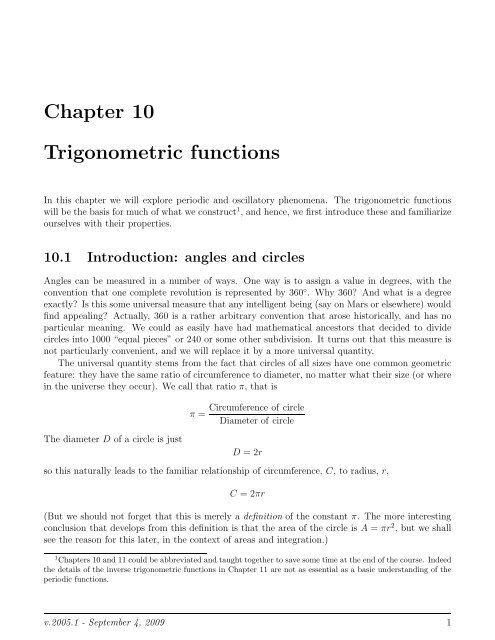
<strong>Chapter</strong> <strong>10</strong><br />
<strong>Trigonometric</strong> <strong>functions</strong><br />
In this chapter we will explore periodic and oscillatory phenomena. The trigonometric <strong>functions</strong><br />
will be the basis for much of what we construct 1 , and hence, we first introduce these and familiarize<br />
ourselves with their properties.<br />
<strong>10</strong>.1 Introduction: angles and circles<br />
Angles <strong>ca</strong>n be measured in a number of ways. One way is to assign a value in degrees, with the<br />
convention that one complete revolution is represented by 360 ◦ . Why 360? And what is a degree<br />
exactly? Is this some universal measure that any intelligent being (say on Mars or elsewhere) would<br />
find appealing? Actually, 360 is a rather arbitrary convention that arose histori<strong>ca</strong>lly, and has no<br />
particular meaning. We could as easily have had <strong>math</strong>emati<strong>ca</strong>l ancestors that decided to divide<br />
circles into <strong>10</strong>00 “equal pieces” or 240 or some other subdivision. It turns out that this measure is<br />
not particularly convenient, and we will replace it by a more universal quantity.<br />
The universal quantity stems from the fact that circles of all sizes have one common geometric<br />
feature: they have the same ratio of circumference to diameter, no matter what their size (or where<br />
in the universe they occur). We <strong>ca</strong>ll that ratio π, that is<br />
π =<br />
Circumference of circle<br />
Diameter of circle<br />
The diameter D of a circle is just<br />
D = 2r<br />
so this naturally leads to the familiar relationship of circumference, C, to radius, r,<br />
C = 2πr<br />
(But we should not forget that this is merely a definition of the constant π. The more interesting<br />
conclusion that develops from this definition is that the area of the circle is A = πr 2 , but we shall<br />
see the reason for this later, in the context of areas and integration.)<br />
1 <strong>Chapter</strong>s <strong>10</strong> and 11 could be abbreviated and taught together to save some time at the end of the course. Indeed<br />
the details of the inverse trigonometric <strong>functions</strong> in <strong>Chapter</strong> 11 are not as essential as a basic understanding of the<br />
periodic <strong>functions</strong>.<br />
v.2005.1 - September 4, 2009 1
Math <strong>10</strong>2 Notes <strong>Chapter</strong> <strong>10</strong><br />
θ<br />
s<br />
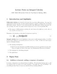
Figure <strong>10</strong>.1: The angle θ in radians is related in a simple way to the radius R of the circle, and the<br />
length of the arc S shown.<br />
From Figure <strong>10</strong>.1 we see that there is a correspondence between the angle (θ) subtended in a<br />
circle of given radius and the length of arc along the edge of the circle. For a circle of radius R and<br />
angle θ we will define the arclength, S by the relation<br />
S = Rθ<br />
where θ is measured in a convenient unit that we will now select. We now consider a circle of radius<br />
R = 1 (<strong>ca</strong>lled a unit circle) and denote by s a length of arc around the perimeter of this unit circle.<br />
In this <strong>ca</strong>se, the arc length is<br />
S = Rθ = θ<br />
We note that when S = 2π, the arc consists of the entire perimeter of the circle. This leads us to<br />
define the unit <strong>ca</strong>lled a radian: we will identify an angle of 2π radians with one complete revolution<br />
around the circle. In other words, we use the length of the arc in the unit circle to assign a numeri<strong>ca</strong>l<br />
value to the angle that it subtends.<br />
We <strong>ca</strong>n now use this choice of unit for angles to assign values to any fraction of a revolution,<br />
and thus, to any angle. For example, an angle of 90 ◦ corresponds to one quarter of a revolution<br />
around the perimeter of a unit circle, so we identify the angle π/2 radians with it. One degree is<br />
1/360 of a revolution, corresponding to 2π/360 radians, and so on.<br />
To summarize our choice of units we have the following two points:<br />
1. The length of an arc along the perimeter of a circle of radius R subtended by an<br />
angle θ is S = Rθ where θ is measured in radians.<br />
2. One complete revolution, or one full cycle corresponds to an angle of 2π radians<br />
It is easy to convert between degrees and radians if we remember that 360 ◦ corresponds to 2π<br />
radians. For example, 180 ◦ then corresponds to π radians, 90 ◦ to π/2 radians, etc.<br />
v.2005.1 - September 4, 2009 2
Math <strong>10</strong>2 Notes <strong>Chapter</strong> <strong>10</strong><br />
<strong>10</strong>.2 Defining the basic trigonometric <strong>functions</strong><br />
(x,y)<br />
t<br />
t<br />
1<br />
x<br />
y<br />
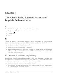
Figure <strong>10</strong>.2: Shown above is the circle of radius 1, x 2 + y 2 = 1. The radius vector that ends at the<br />
point (x, y) subtends an angle t (radians) with the x axis. The triangle is also shown enlarged to<br />
the right, where the lengths of all three sides is labeled. The trigonometric <strong>functions</strong> are just ratios<br />
of two sides of this triangle.<br />
hypotenuse<br />
θ<br />
adjacent<br />
opposite<br />
sin θ = opp/hyp<br />
cos θ =adj/hyp<br />
tan θ=opp/adj<br />
Figure <strong>10</strong>.3: Review of the relation between ratios of side lengths (in a right triangle) and trigonometric<br />
<strong>functions</strong> of the associated angle.<br />
Consider a point (x, y) on a circle of radius 1, and let t be some angle (measured in radians)<br />
formed by the x axis and the radius vector to the point (x, y) as shown in Figure <strong>10</strong>.2.<br />
We will define two new <strong>functions</strong>, sine and cosine (abbreviated sin and cos) as follows:<br />
sin(t) = y 1 = y,<br />
cos(t) = x 1 = x<br />
That is, the function sine tracks the y coordinate of the point as it moves around the unit circle, and<br />
the function cosine tracks its x coordinate. (Remark: this agrees with previous definitions of these<br />
trigonometric quantities as shown in Figure <strong>10</strong>.3 as the opposite over hypotenuse and adjacent over<br />
hypotenuse in a right angle triangle that you may have encountered in high school. The hypotenuse<br />
in our diagram is simply the radius of the circle, which is 1 by assumption.)<br />
v.2005.1 - September 4, 2009 3
Math <strong>10</strong>2 Notes <strong>Chapter</strong> <strong>10</strong><br />
<strong>10</strong>.3 Properties of the trigonometric <strong>functions</strong><br />
We now explore the consequences of these definitions:<br />
Values of sine and cosine<br />
• The radius of the circle is 1. This means that the x coordinate <strong>ca</strong>nnot be larger than 1 or<br />
smaller than -1. Same holds for the y coordinate. Thus the <strong>functions</strong> sin(t) and cos(t) are<br />
always swinging between -1 and 1. (−1 ≤ sin(t) ≤ 1 and −1 ≤ cos(t) ≤ 1 for all t). The peak<br />
(maximum) value of each function is 1, the minimum is -1, and the average value is 0.<br />
• When the radius vector points along the x axis, the angle is t = 0 and we have y = 0, x = 1.<br />
This means that cos(0) = 1, sin(0) = 0.<br />
• When the radius vector points up the y axis, the angle is π/2 (corresponding to one quarter<br />
of a complete revolution), and here x = 0, y = 1 so that cos(π/2) = 0, sin(π/2) = 1.<br />
• Using simple geometry, we <strong>ca</strong>n also determine the lengths of all sides, and hence the ratios of<br />
the sides in a few particularly simple triangles, namely triangles (in which all angles are 60 ◦ ),<br />
and right triangles with two equal angles of 45 ◦ . These types of <strong>ca</strong>lculations (omitted here)<br />
lead to some easily determined values for the sine and cosine of such special angles. These<br />
values are shown in the table below.<br />
degrees radians sin(t) cos(t) tan(t)<br />
0 0 0 1 0<br />
π<br />
30<br />
6<br />
π<br />
45<br />
4<br />
Connection between sine and cosine<br />
1<br />
√2<br />
2<br />
√2<br />
3<br />
2<br />
√<br />
3 1√<br />
√2<br />
3<br />
2<br />
2<br />
1<br />
√<br />
π<br />
1<br />
60<br />
3<br />
2 3<br />
π<br />
90<br />
2<br />
1 0 ∞<br />
• The two <strong>functions</strong>, sine and cosine depict the same underlying motion, viewed from two<br />
perspectives: cos(t) represents the projection of the circularly moving point onto the x axis,<br />
while sin(t) is the projection of that point onto the y axis. In this sense, the <strong>functions</strong> are a<br />
pair of twins, and we <strong>ca</strong>n expect many relationships to hold between them.<br />
• The cosine has its largest value at the beginning of the cycle, when t = 0 (since cos(0) = 1),<br />
while the other the sine its peak value a little later, (sin(π/2) = 1). Throughout their circular<br />
race, the sine function is π/2 radians ahead of the cosine i.e.<br />
cos(t) = sin(t + π 2 ).<br />
• The point (x, y) is on a circle of radius 1, and, thus, its coordinates satisfy<br />
x 2 + y 2 = 1<br />
v.2005.1 - September 4, 2009 4
Math <strong>10</strong>2 Notes <strong>Chapter</strong> <strong>10</strong><br />
1<br />
0.5<br />
0<br />
2 4 6 8 <strong>10</strong> 12<br />
t<br />
–0.5<br />
–1<br />
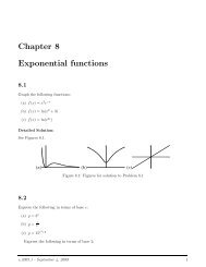
Figure <strong>10</strong>.4: The <strong>functions</strong> sin(t) and cos(t) are periodic, that is, they have a basic pattern that<br />
repeats. The two <strong>functions</strong> are also related, since one is just a copy of the other, shifted along the<br />
x axis.<br />
This implies that<br />
sin 2 (t) + cos 2 (t) = 1<br />
for any angle t. This is an important relation, (also <strong>ca</strong>lled an identity between the two<br />
trigonometric <strong>functions</strong>, and one that we will use quite often.<br />
Periodicity: the pattern repeats<br />
• A function is said to be periodic if its graph is repeated over and over again. For example, if<br />
the basic shape of the graph occurs in an interval of length T on the t axis, and this shape is<br />
repeated, then it would be true that<br />
f(t) = f(t + T).<br />
In this <strong>ca</strong>se we <strong>ca</strong>ll T the period of the function. All the trigonometric <strong>functions</strong> are periodic.<br />
• The point (x, y) in Figure <strong>10</strong>.2 will repeat its trajectory every time a revolution around the<br />
circle is complete. This happens when the angle t completes one full cycle of 2π radians.<br />
Thus, as expected, the trigonometric <strong>functions</strong> are periodic, that is<br />
We say that the period is T = 2π radians.<br />
sin(t) = sin(t + 2π),<br />
cos(t) = cos(t + 2π).<br />
We <strong>ca</strong>n make other observations about the same two <strong>functions</strong>. For example, by noting the<br />
symmetry of the <strong>functions</strong> relative to the origin, we <strong>ca</strong>n see that sin(t) is an odd function and<br />
the cos(t) is an even function. This follows from the fact that for a negative angle (i.e. an angle<br />
clockwise from the x axis) the sine flips sign while the cosine does not.<br />
v.2005.1 - September 4, 2009 5
Math <strong>10</strong>2 Notes <strong>Chapter</strong> <strong>10</strong><br />
1<br />
y=sin (t)<br />
0<br />
−1<br />
π/2 π 3π/2 2π 5π/2<br />
3π<br />
t<br />
period, T<br />
y=cos (t)<br />
1<br />
0<br />
π/2 π 3π/2 2π 5π/2 3π<br />
t<br />
−1<br />
period, T<br />
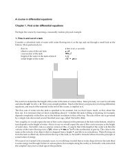
Figure <strong>10</strong>.5: Periodicity of the sine and cosine. Note that the two curves are just shifted versions<br />
of one another.<br />
<strong>10</strong>.4 Phase, amplitude, and frequency<br />
We have already learned how the appearance of <strong>functions</strong> changes when we shift their graph in<br />
one direction or another, s<strong>ca</strong>le one of the axes, and so on. Thus it will be easy to follow the basic<br />
changes in shape of a typi<strong>ca</strong>l trigonometric function.<br />
A function of the form<br />
y = f(t) = A sin(ωt)<br />
has both its t and y axes s<strong>ca</strong>led. The constant A, referred to as the amplitude of the graph, s<strong>ca</strong>les<br />
the y axis so that the oscillation swings between a low value of −A and a high value of A. The<br />
constant ω, <strong>ca</strong>lled the frequency, s<strong>ca</strong>les the t axis. This results in crowding together of the peaks<br />
and valleys (if ω > 1) or stretching them out (if ω < 1). One full cycle is completed when<br />
ωt = 2π<br />
and this occurs at time<br />
t = 2π ω .<br />
We will use the symbol T, to denote this special time, and we refer to T as the period. We note the<br />
connection between frequency and period:<br />
ω = 2π<br />
T ,<br />
T = 2π ω .<br />
v.2005.1 - September 4, 2009 6
Math <strong>10</strong>2 Notes <strong>Chapter</strong> <strong>10</strong><br />
2.0<br />
y=sin(t)<br />
2.0<br />
y=Asin(t)<br />
-2.0<br />
0.0 6.3<br />
-2.0<br />
0.0 6.3<br />
2.0<br />
2.0<br />
y=A sin(w t)<br />
y=A sin(w (t-a))<br />
-2.0<br />
0.0 6.3<br />
-2.0<br />
0.0 6.3<br />
Figure <strong>10</strong>.6: Graphs of the <strong>functions</strong> (a) y = sin(t), (b) y = A sin(t) A > 1, (c) y = A sin(ωt) ω > 1,<br />
(d) y = A sin(ω(t − a)).<br />
If we examine a graph of function<br />
y = f(t) = A sin(ω(t − a))<br />
we find that the graph has been shifted in the positive t direction by a. We note that at time t = a,<br />
the value of the function is<br />
y = f(t) = A sin(ω(a − a)) = A sin(0) = 0.<br />
This tells us that the cycle “starts” with a delay, i.e. the value of y goes through zero when when<br />
t = a.<br />
Another common variant of the same function <strong>ca</strong>n be written in the form<br />
y = f(t) = A sin(ωt − φ).<br />
Here φ is <strong>ca</strong>lled the phase shift of the oscillation. Comparing the above two related forms, we see<br />
that they are the same if we identify φ with ωa. The phase shift, φ is considered to be a quantity<br />
v.2005.1 - September 4, 2009 7
Math <strong>10</strong>2 Notes <strong>Chapter</strong> <strong>10</strong><br />
without units, whereas the quantity a has units of time, same as t. When φ = 2π, (which is the<br />
same as the <strong>ca</strong>se that a = 2π/ω, the graph has been moved over to the right by one full period.<br />
(Naturally, when the graph is so moved, it looks the same as it did originally, since each cycle is<br />
the same as the one before, and same as the one after.)<br />
Some of the s<strong>ca</strong>led, shifted, sine <strong>functions</strong> described here are shown in Figure <strong>10</strong>.6.<br />
<strong>10</strong>.5 Rhythmic processes<br />
Many natural phenomena are cyclic. It is often convenient to represent such phenomena with one<br />
or another simple periodic <strong>functions</strong>, and sine and cosine <strong>ca</strong>n be adapted for the purpose. The idea<br />
is to pick the right function , the right frequency (or period), the amplitude, and possibly the phase<br />
shift, so as to represent the desired behaviour.<br />
To select one or another of these <strong>functions</strong>, it helps to remember that cosine starts a cycle (at<br />
t = 0) at its peak value, while sine starts the cycle at 0, i.e., at its average value. A function that<br />
starts at the lowest point of the cycle is − cos(t). In most <strong>ca</strong>ses, the choice of function to use is<br />
somewhat arbitrary, since a phase shift <strong>ca</strong>n correct for the phase at which the oscillation starts.<br />
Next, we pick a constant ω such that the trigonometric function sin(ωt) (or cos(ωt)) has the<br />
correct period. Given a period for the oscillation, T, re<strong>ca</strong>ll that the corresponding frequency is<br />
simply ω = 2π . We then select the amplitude, and horizontal and verti<strong>ca</strong>l shifts to complete the<br />
T<br />
mission. The examples below illustrate this process.<br />
Example 1: daylight hours<br />
In Vancouver, the shortest day (8 hours of light) occurs around December 22, and the longest day<br />
(16 hours of light) is around June 21. Approximate the cyclic changes of daylight through the<br />
season using the sine function.<br />
Solution:<br />
On Sept 21 and March 21 the lengths of day and night are equal, and then there are 12 hours<br />
of daylight. (Each of these days is <strong>ca</strong>lled an equinox). Suppose we <strong>ca</strong>ll identify March 21 as the<br />
beginning of a yearly day-night length cycle. Let t be time in days beginning on March 21. One<br />
full cycle takes a year, i.e. 365 days. The period of the function we want is thus<br />
and its frequency is<br />
T = 365<br />
ω = 2π/365.<br />
Daylight shifts between the two extremes of 8 and 16 hours: i.e. 12 ± 4 hours. This means that the<br />
amplitude of the cycle is 4 hours. The oscillation take place about the average value of 12 hours.<br />
We have decided to start a cycle on a day for which the number of daylight hours is the average<br />
value (12). This means that the sine would be most appropriate, so the function that best describes<br />
the number of hours of daylight at different times of the year is:<br />
( ) 2π<br />
D(t) = 12 + 4 sin<br />
365 t<br />
where t is time in days and D the number of hours of light.<br />
v.2005.1 - September 4, 2009 8
Math <strong>10</strong>2 Notes <strong>Chapter</strong> <strong>10</strong><br />
Example 2: hormone levels<br />
The level of a certain hormone in the bloodstream fluctuates between undetectable concentration<br />
at 7:00 and <strong>10</strong>0 ng/ml at 19:00 hours. Approximate the cyclic variations in this hormone level<br />
with the appropriate periodic trigonometric function. Let t represent time in hours from 0:00 hrs<br />
through the day.<br />
Solution:<br />
<strong>10</strong>0<br />
H(t)<br />
period: T= 24 hrs<br />
50<br />
t<br />
0 1 7 13 19<br />
24<br />
12 hrs<br />
6 hrs<br />
Figure <strong>10</strong>.7: Hormonal cycles. The full cycle is 24 hrs. The level H(t) swings between 0 and <strong>10</strong>0<br />
ng. From the given information, we see that the average level is 50 ng, and that the origin of a<br />
representative sine curve should be at t = 13 (i.e. 1/4 of the cycle which is 6 hrs past the time<br />
point t = 7) to depict this cycle.<br />
We first note that it takes one day (24 hours) to complete a cycle. This means that the period<br />
of oscillation is 24 hours, so that the frequency is<br />
ω = 2π<br />
T = 2π<br />
24 = π 12 .<br />
The variation in the level of hormone is between 0 and <strong>10</strong>0 ng/ml, which <strong>ca</strong>n be expressed as 50<br />
± 50 ng/ml. (The trigonometric <strong>functions</strong> are symmetric cycles, and we are here finding both the<br />
average value about which cycles occur and the amplitude of the cycles.) We could consider the<br />
time midway between the low and high points, namely 13:00 hours as the point corresponding to<br />
the upswing at the start of a cycle of the sine function. (See Figure <strong>10</strong>.7 for the sketch.) Thus, if<br />
we use a sine to represent the oscillation, we should shift it by 13 hrs to the left. Assembling these<br />
observations, we obtain the level of hormone, H at time t in hours:<br />
( π<br />
)<br />
H(t) = 50 + 50 sin<br />
12 (t − 13) .<br />
v.2005.1 - September 4, 2009 9
Math <strong>10</strong>2 Notes <strong>Chapter</strong> <strong>10</strong><br />
In the expression above, the number 13 represents a shift along the time axis, and <strong>ca</strong>rries units of<br />
time. We <strong>ca</strong>n express this same function in the form<br />
( πt<br />
H(t) = 50 + 50 sin<br />
12 − 13π )<br />
.<br />
12<br />
In this version, the quantity<br />
φ = 13π<br />
12<br />
is what we have referred to as a phase shift. (This represents the point on the 2π cycle at which<br />
the function begins when we plug in t = 0.)<br />
In selecting the periodic function to use for this example, we could have made other choices.<br />
For example, the same periodic <strong>ca</strong>n be represented by any of the <strong>functions</strong> listed below:<br />
( π<br />
)<br />
H(t) = 50 − 50 sin<br />
12 (t − 1) ,<br />
( π<br />
)<br />
H(t) = 50 + 50 cos<br />
12 (t − 19) ,<br />
( π<br />
)<br />
H(t) = 50 − 50 cos<br />
12 (t − 7) .<br />
All these <strong>functions</strong> have the same values, the same amplitudes, and the same periods.<br />
Example 3: phases of the moon<br />
0 29.5<br />
Figure <strong>10</strong>.8: Periodic moon phases<br />
A cycle of waxing and waning moon takes 29.5 days approximately. Construct a periodic function<br />
to describe the changing phases, starting with a “new moon” (totally dark) and ending one cycle<br />
later.<br />
Solution:<br />
The period of the cycle is T = 29.5 days, so<br />
ω = 2π<br />
T = 2π<br />
29.5 .<br />
v.2005.1 - September 4, 2009 <strong>10</strong>
Math <strong>10</strong>2 Notes <strong>Chapter</strong> <strong>10</strong><br />
For this example, we will use the cosine function, for practice. Let P(t) be the fraction of the moon<br />
showing on day t in the cycle. Then we should construct the function so that 0 < P < 1, with<br />
P = 1 in mid cycle (see Figure <strong>10</strong>.8). The cosine function swings between the values -1 and 1. To<br />
obtain a positive function in the desired range for P(t), we will add a constant and s<strong>ca</strong>le the cosine<br />
as follows:<br />
1<br />
[1 + cos(ωt)].<br />
2<br />
This is not quite right, though be<strong>ca</strong>use at t = 0 this function takes the value 1, rather than 0, as<br />
shown in Figure <strong>10</strong>.8. To correct this we <strong>ca</strong>n either introduce a phase shift, i.e. set<br />
P(t) = 1 [1 + cos(ωt + π)].<br />
2<br />
(Then when t = 0, we get P(t) = 0.5[1 + cosπ] = 0.5[1 − 1] = 0.) or we <strong>ca</strong>n write<br />
which achieves the same result.<br />
P(t) = 1 [1 − cos(ωt + π)],<br />
2<br />
<strong>10</strong>.6 Other trigonometric <strong>functions</strong><br />
Although we shall mostly be concerned with the two basic <strong>functions</strong> described above, several others<br />
are histori<strong>ca</strong>lly important and are encountered frequently in integral <strong>ca</strong>lculus. These include the<br />
following:<br />
tan(t) = sin(t)<br />
cos(t) , cot(t) = 1<br />
tan(t) ,<br />
The identity<br />
sec(t) = 1<br />
cos(t) , csc(t) = 1<br />
sin(t) .<br />
sin 2 (t) + cos 2 (t) = 1<br />
then leads to two others of similar form. Dividing each side of the above relation by cos 2 (t) yields<br />
whereas division by sin 2 (t) gives us<br />
tan 2 (t) + 1 = sec 2 (t)<br />
1 + cot 2 (t) = csc 2 (t).<br />
These will be important for simplifying expressions involving the trigonometric <strong>functions</strong>, as we<br />
shall see.<br />
Law of cosines<br />
This law relates the cosine of an angle to the lengths of sides formed in a triangle. (See figure <strong>10</strong>.9.)<br />
c 2 = a 2 + b 2 − 2ab cos(θ)<br />
where the side of length c is opposite the angle θ.<br />
Here are other important relations between the trigonometric <strong>functions</strong> that should be remembered.<br />
These are <strong>ca</strong>lled trigonometric identities:<br />
v.2005.1 - September 4, 2009 11
Math <strong>10</strong>2 Notes <strong>Chapter</strong> <strong>10</strong><br />
b<br />
θ<br />
c<br />
a<br />
Figure <strong>10</strong>.9:<br />
Angle sum identities<br />
The trigonometric <strong>functions</strong> are nonlinear. This means that, for example, the sine of the sum of<br />
two angles is not just the sum of the two sines. One <strong>ca</strong>n use the law of cosines and other geometric<br />
ideas to establish the following two relationships:<br />
sin(A + B) = sin(A) cos(B) + sin(B) cos(A)<br />
cos(A + B) = cos(A) cos(B) − sin(A) sin(B)<br />
These two identities appear in many <strong>ca</strong>lculations, and will be important for computing derivatives<br />
of the basic trigonometric formulae.<br />
Related identities<br />
The identities for the sum of angles <strong>ca</strong>n be used to derive a number of related formulae. For example,<br />
by replacing B by −B we get the angle difference identities:<br />
sin(A − B) = sin(A) cos(B) − sin(B) cos(A)<br />
cos(A − B) = cos(A) cos(B) + sin(A) sin(B)<br />
By setting θ = A = B in these we find the subsidiary double angle formulae:<br />
and these <strong>ca</strong>n also be written in the form<br />
sin(2θ) = 2 sin(θ) cos(θ)<br />
cos(2θ) = cos 2 (θ) − sin 2 (θ)<br />
2 cos 2 (θ) = 1 + cos(2θ)<br />
2 sin 2 (θ) = 1 − cos(2θ).<br />
(The latter four are quite useful in integration methods.)<br />
v.2005.1 - September 4, 2009 12
Math <strong>10</strong>2 Notes <strong>Chapter</strong> <strong>10</strong><br />
<strong>10</strong>.7 Limits involving the trigonometric <strong>functions</strong><br />
Before we compute derivatives of the sine and cosine <strong>functions</strong> using the definition of the derivative,<br />
we will need to specify two limits that will be needed in those <strong>ca</strong>lculations.<br />
1<br />
0.8<br />
0.6<br />
0.4<br />
0.5<br />
0.4<br />
0.2<br />
0.2<br />
–3 –2 –1 0 1 2 3 –1 –0.8 –0.6 –0.4 –0.2 0 0.2 0.4 0.6 0.8 1<br />
–0.4 –0.2 0 0.2 0.4<br />
x<br />
–0.2<br />
x<br />
x<br />
–0.5<br />
–0.4<br />
–0.2<br />
–1<br />
–0.6<br />
–0.8<br />
–0.4<br />
Figure <strong>10</strong>.<strong>10</strong>: Zooming in on the graph of y = sin(x) at x = 0<br />
If we zoom in on the graph of the sine function close to the origin, we will see a curve resembling<br />
a straight line with slope 1, i.e. the function y = sin(t) will look quite similar to the graph of y = t<br />
close to t = 0. This is shown in the sequence of graphs in Figure <strong>10</strong>.<strong>10</strong>. This means that, for small<br />
t<br />
sin(t) ≈ t.<br />
We <strong>ca</strong>n restate this as<br />
sin(h) ≈ h<br />
or as<br />
sin(h)<br />
≈ 1.<br />
h<br />
It turns out that this approximation becomes finer as h decreases, i.e<br />
sin(h)<br />
lim<br />
h→0 h<br />
This is a very important limit, and will be used in many appli<strong>ca</strong>tions.<br />
A similar analysis of the graph of the cosine function, shown in Figure <strong>10</strong>.11, will lead us to<br />
conclude that the related limit is<br />
cos(h) − 1<br />
lim = 0.<br />
h→0 h<br />
We <strong>ca</strong>n now apply these to computing derivatives.<br />
= 1.<br />
<strong>10</strong>.7.1 Derivatives of the trigonometric <strong>functions</strong><br />
Let y = f(x) = sin(x) be the function to differentiate, where x is now the independent variable<br />
(previously <strong>ca</strong>lled t). Below, we use the definition of the derivative to compute the derivative of<br />
this function.<br />
v.2005.1 - September 4, 2009 13
Math <strong>10</strong>2 Notes <strong>Chapter</strong> <strong>10</strong><br />
1<br />
1<br />
1<br />
0.8<br />
0.8<br />
0.5<br />
0.6<br />
0.6<br />
z<br />
z<br />
–3 –2 –1 0 1 2 3<br />
x<br />
0.4<br />
0.4<br />
–0.5<br />
0.2<br />
0.2<br />
–1 –0.8 –0.6 –0.4 –0.2 0 0.2 0.4 0.6 0.8 1 –0.2 –0.1 0<br />
0.1 0.2<br />
–1<br />
x<br />
x<br />
Figure <strong>10</strong>.11: Zooming in on the graph of y = cos(x) at x = 0<br />
f ′ f(x + h) − f(x)<br />
(x) = lim<br />
h→0 h<br />
d sin(x) sin(x + h) − sin(x)<br />
= lim<br />
dx h→0 h<br />
sin(x) cos(h) + sin(h) cos(x) − sin(x)<br />
= lim<br />
h→0<br />
(<br />
h<br />
= lim sin(x) cos(h) − 1 + cos(x) sin(h) )<br />
h→0 h<br />
h<br />
( ) ( )<br />
cos(h) − 1<br />
sin(h)<br />
= sin(x) lim + cos(x) lim<br />
h→0 h<br />
h→0 h<br />
= cos(x) (<strong>10</strong>.1)<br />
Observe that the limits described in the preceding section were used in getting to our final result.<br />
A similar <strong>ca</strong>lculation using the function cos(x) leads to the result<br />
d cos(x)<br />
dx<br />
= − sin(x).<br />
(The same two limits appear in this <strong>ca</strong>lculation as well.)<br />
We <strong>ca</strong>n now <strong>ca</strong>lculate the derivative of the any of the other trigonometric <strong>functions</strong> using the<br />
quotient rule. For example, let us consider the derivative of y = tan(x):<br />
v.2005.1 - September 4, 2009 14
Math <strong>10</strong>2 Notes <strong>Chapter</strong> <strong>10</strong><br />
d tan(x)<br />
dx<br />
= [sin(x)]′ cos(x) − [cos(x)] ′ sin(x)<br />
cos 2 (x)<br />
Using the recently found derivatives for the sine and cosine, we have<br />
d tan(x)<br />
dx<br />
= sin2 (x) + cos 2 (x)<br />
.<br />
cos 2 (x)<br />
But the numerator of the above <strong>ca</strong>n be simplified using the trigonometric identity, leading<br />
to<br />
d tan(x) 1<br />
=<br />
dx cos 2 (x) = sec2 (x).<br />
The derivatives of the six trigonometric <strong>functions</strong> are given in the table below. The reader may<br />
wish to practice the use of the quotient rule by verifying one or more of the derivatives of the<br />
relatives csc(x) or sec(x). In practice, the most important <strong>functions</strong> are the first three, and their<br />
derivatives should be remembered, as they are frequently encountered in practi<strong>ca</strong>l appli<strong>ca</strong>tions.<br />
y = f(x)<br />
sin(x)<br />
cos(x)<br />
tan(x)<br />
csc(x)<br />
sec(x)<br />
cot(x)<br />
f ′ (x)<br />
cos(x)<br />
− sin(x)<br />
sec 2 (x)<br />
− csc(x) cot(x)<br />
sec(x) tan(x)<br />
− csc 2 (x)<br />
<strong>10</strong>.8 <strong>Trigonometric</strong> related rates<br />
The examples in this section will allow us to practice chain rule appli<strong>ca</strong>tions using the trigonometric<br />
<strong>functions</strong>. We will discuss a number of problems, and show how the basic facts described in this<br />
chapter appear in various combinations to arrive at desired results.<br />
Example 1:<br />
A point moves around the rim of a circle of radius 1 so that the angle θ subtended by the radius<br />
vector to that point changes at a constant rate,<br />
θ = ωt,<br />
where t is time. Determine the rate of change of the x and y coordinates of that point.<br />
Solution:<br />
We have θ(t), x(t), and y(t) all <strong>functions</strong> of t. The fact that θ is proportional to t means that<br />
dθ<br />
dt = ω.<br />
The x and y coordinates of the point are related to the angle by<br />
x(t) = cos(θ(t)) = cos(ωt),<br />
v.2005.1 - September 4, 2009 15
Math <strong>10</strong>2 Notes <strong>Chapter</strong> <strong>10</strong><br />
This implies (by the chain rule) that<br />
Performing the required <strong>ca</strong>lculations, we have<br />
y(t) = sin(θ(t)) = sin(ωt).<br />
dx<br />
dt = d cos(θ) dθ<br />
dθ dt ,<br />
dy<br />
dt = d sin(θ) dθ<br />
dθ dt .<br />
dx<br />
dt = − sin(θ)ω,<br />
dy<br />
dt = cos(θ)ω.<br />
We will see some interesting consequences of this in a later section.<br />
Example 2: runners on a circular track<br />
Two runners start at the same position (<strong>ca</strong>ll it x = 0) on a circular race track of length 400 meters.<br />
Joe Runner takes 50 sec, while Michael Johnson takes 43.18 sec to complete the 400 meter race.<br />
Determine the rate of change of the angle formed between the two runners and the center of the<br />
track, assuming that the runners are running at a constant rate.<br />
Solution:<br />
The track is 400 meters in length (total). Joe completes one cycle around the track (2π radians) in<br />
50 sec, while Michael completes a cycle in 43.18 sec. (This means that Joe has period of T = 50 sec,<br />
and a frequency of ω 1 = 2π/T = 2π/50 radians per sec. Similarly, Michael’s period is T = 43.18<br />
sec and his frequency is ω 2 = 2π/T = 2π/43.18 radians per sec. From this, we find that<br />
dθ J<br />
dt = 2π<br />
50<br />
dθ M<br />
dt<br />
= 0.125 radians per sec<br />
= 2π = 0.145 radians per sec<br />
43.18<br />
Thus the angle between the runners, θ M − θ J changes at the rate<br />
d(θ M − θ J )<br />
dt<br />
= 0.145 − 0.125 = 0.02 radians per sec<br />
Example 3: simple law of cosines<br />
Consider the triangle as shown in Figure <strong>10</strong>.9. Suppose that the angle θ increases at a constant<br />
rate, i.e. dθ/dt = k. If the sides a = 3, b = 4, are of constant length, determine the rate of change<br />
of the length c opposite this angle at the instant that c = 5.<br />
v.2005.1 - September 4, 2009 16
Math <strong>10</strong>2 Notes <strong>Chapter</strong> <strong>10</strong><br />
Solution:<br />
Let a, b, c be the lengths of the three sides, with c the length of the side opposite angle θ. The law<br />
of cosines states that<br />
c 2 = a 2 + b 2 − 2ab cos(θ).<br />
We identify the changing quantities by writing this relation in the form<br />
c 2 (t) = a 2 + b 2 − 2ab cos(θ(t))<br />
so it is evident that only c and θ will vary with time, while a, b remain constant. We are also told<br />
that<br />
dθ<br />
dt = k.<br />
Differentiating and using the chain rule leads to:<br />
But d cos(θ)/dθ = − sin(θ) so that<br />
2c dc<br />
dt<br />
cos(θ) dθ<br />
= −2abd<br />
dθ dt<br />
dc<br />
dt = −ab (− sin(θ))dθ<br />
c dt = ab<br />
c k sin(θ).<br />
We now note that at the instant in question, a = 3, b = 4, c = 5, forming a Pythagorean triangle<br />
in which the angle opposite c is θ = π/2. We <strong>ca</strong>n see this fact using the law of cosines, and noting<br />
that<br />
c 2 = a 2 + b 2 − 2ab cos(θ), 25 = 9 + 16 − 24 cos(θ).<br />
This implies that 0 = −24 cos(θ), cos(θ) = 0 so that θ = π/2. Substituting these into our result for<br />
the rate of change of the length c leads to<br />
Example 4: clocks<br />
dc<br />
dt = ab<br />
c k = 3 · 4<br />
5 k.<br />
(a) Find the rate of change of the angle between the minute hand and hour hand on a clock.<br />
(b) Suppose that the length of the minute hand is 4 cm and the length of the hour hand is 3<br />
cm. At what rate is the distance between the hands changing when it is 3:00 o’clock?<br />
Solution to (a):<br />
We will <strong>ca</strong>ll θ 1 the angle that the minute hand subtends with the x axis (horizontal direction) and<br />
θ 2 the angle that the hour hand makes with the same axis.<br />
If our clock is working properly, each hand will move around at a constant rate. The hour hand<br />
will trace out one complete revolution (2π radians) every 12 hours, while the minute hand will<br />
complete a revolution every hour. Both hands move in a clockwise direction, which (by convention)<br />
is towards negative angles. This means that<br />
dθ 1<br />
dt<br />
= −2π radians per hour,<br />
v.2005.1 - September 4, 2009 17
Math <strong>10</strong>2 Notes <strong>Chapter</strong> <strong>10</strong><br />
θ<br />
1<br />
θ<br />
2<br />
x<br />
Figure <strong>10</strong>.12:<br />
dθ 2<br />
dt = −2π radians per hour.<br />
12<br />
The angle between the two hands is the difference of the two angles, i.e.<br />
θ = θ 1 − θ 2<br />
Thus,<br />
dθ<br />
dt = d dt (θ 1 − θ 2 ) = dθ 1<br />
dt − dθ 2 2π<br />
= −2π +<br />
dt 12<br />
Thus, we find that the rate of change of the angle between the hands is<br />
dθ<br />
dt = −2π11 12 = −π11 6 .<br />
θ −θ<br />
1<br />
2<br />
x<br />
Figure <strong>10</strong>.13:<br />
Solution to (b):<br />
We use the law of cosines to give us the rate of change of the desired distance. We have the triangle<br />
shown in figure <strong>10</strong>.12 in which side lengths are a = 3, b = 4, and c(t) opposite the angle θ(t). From<br />
v.2005.1 - September 4, 2009 18
Math <strong>10</strong>2 Notes <strong>Chapter</strong> <strong>10</strong><br />
the previous example, we have<br />
dc<br />
dt = ab<br />
c sin(θ)dθ dt .<br />
At precisely 3:00 o’clock, the angle in question is θ = π/2 and it <strong>ca</strong>n also be seen that the<br />
Pythagorean triangle abc leads to<br />
c 2 = a 2 + b 2 = 3 2 + 4 2 = 9 + 16 = 25<br />
so that c = 5. We found from our previous analysis that dθ/dt = 11 π. Using this information leads<br />
6<br />
to:<br />
dc<br />
dt = 3 · 4<br />
5 sin(π/2)(−11 6 π) = −22 π cm per hr<br />
5<br />
The negative sign indi<strong>ca</strong>tes that at this time, the distance between the two hands is decreasing.<br />
Example 5: visual angles<br />
θ<br />
x<br />
S<br />
Figure <strong>10</strong>.14:<br />
In the triangle shown in Figure <strong>10</strong>.14, an object of height s is moving towards an observer. Its<br />
distance from the observer at some instant is labeled x(t) and it approaches at some constant speed,<br />
v. We would like to relate the rate of change of the angle θ(t) to the speed, size, and distance of<br />
the object. Often θ is <strong>ca</strong>lled a visual angle, since it represents the angle that an image subtends on<br />
the retina of the observer. A more detailed example of this type is discussed in the next chapter.<br />
Solution:<br />
We are given the information that the object approaches at some constant speed, v. This means<br />
that<br />
dx<br />
dt = −v.<br />
(The minus sign means that the distance x is decreasing.) Using the trigonometric relations, we see<br />
that<br />
tan(θ) = s x .<br />
If the size, s, of the object is constant, then the changes with time imply that<br />
tan(θ(t)) =<br />
s<br />
x(t) .<br />
v.2005.1 - September 4, 2009 19
Math <strong>10</strong>2 Notes <strong>Chapter</strong> <strong>10</strong><br />
We differentiate both sides of this equation with respect to t, and obtain<br />
d tan(θ) dθ<br />
dθ dt = d ( ) s<br />
dt x(t)<br />
so that<br />
We <strong>ca</strong>n use the trigonometric identity<br />
sec 2 (θ) dθ<br />
dt = −s 1 dx<br />
x 2 dt<br />
dθ<br />
dt = −s 1<br />
sec 2 (θ)<br />
1 dx<br />
x 2 dt<br />
sec 2 (θ) = 1 + tan 2 (θ)<br />
to express our answer in terms only of the size, s, the distance of the object, x and the speed:<br />
so<br />
( s 2<br />
sec 2 x<br />
(θ) = 1 + =<br />
x) 2 + s 2<br />
dθ<br />
dt = −s x 2<br />
x 2 + s 2 1<br />
x 2 dx<br />
dt =<br />
x 2<br />
S<br />
x 2 + s 2v.<br />
(Two minus signs <strong>ca</strong>ncelled above.) Thus, the rate of change of the visual angle is sv/(x 2 + s 2 ).<br />
This <strong>ca</strong>lculation has some interesting impli<strong>ca</strong>tions for reactions to visual stimuli. We will explore<br />
some of these impli<strong>ca</strong>tions later on.<br />
<strong>10</strong>.9 <strong>Trigonometric</strong> <strong>functions</strong> and differential equations<br />
In this section, we will show the following relationship between trigonometric <strong>functions</strong> and differential<br />
equations:<br />
The <strong>functions</strong><br />
x(t) = cos(ωt), y(t) = sin(ωt)<br />
satisfy a pair of differential equations,<br />
dx<br />
dt = −ωy,<br />
dy<br />
dt = ωx.<br />
The <strong>functions</strong><br />
x(t) = cos(ωt),<br />
y(t) = sin(ωt)<br />
also satisfy a related differential equation with a second derivative<br />
d 2 x<br />
dt 2 = −ω2 x.<br />
To show that these statements are true, we return to an example explored in the previous section:<br />
we considered a point moving around a unit circle at a constant angular rate, ω, so that<br />
dθ<br />
dt = ω.<br />
v.2005.1 - September 4, 2009 20
Math <strong>10</strong>2 Notes <strong>Chapter</strong> <strong>10</strong><br />
We then considered the x and y coordinates of the point,<br />
x(t) = cos(θ(t)) = cos(ωt),<br />
y(t) = sin(θ(t)) = sin(ωt),<br />
and showed (using the chain rule) that these satisfy<br />
dx<br />
dt = − sin(θ)ω,<br />
dy<br />
dt = cos(θ)ω.<br />
These relationships <strong>ca</strong>n also be written in the form<br />
dx<br />
dt = −ωy,<br />
dy<br />
dt = ωx,<br />
where we have used the definitions of sine and cosine in terms of x and y.<br />
The above pair of equations describe the fact that the derivative of each of these trig <strong>functions</strong>,<br />
x(t) and y(t), is related to the other function. These two equations fall into a class we have already<br />
explored, namely differential equations.<br />
We have just shown that the <strong>functions</strong> x(t) = cos(ωt) and y(t) = sin(ωt) also have a special<br />
connection to differential equations. In fact they are linked by the pair of interconnected equations<br />
displayed here as our result. Each equation involves the derivative of one or the other of the trig<br />
<strong>functions</strong>, and says that this derivative is just a constant multiple of the other function. (In a way, we<br />
already knew this relationship holds, since our table of derivatives illustrates the connection between<br />
sin and cos. However, we here see the idea in a setting that reminds us of similar observations made<br />
for exponential <strong>functions</strong>. (Such interdependent differential equations are also referred to as a set<br />
of coupled equations, since each one contains variables that appear in the other.)<br />
By differentiating both sides of the first equation, we find that<br />
d 2 x<br />
dt 2 = −ωdy dt ,<br />
and now using the second equation, we simplify to<br />
d 2 x<br />
dt 2 = −ω(ωx),<br />
finally obtaining<br />
d 2 x<br />
dt = 2 −ω2 x.<br />
The reader <strong>ca</strong>n show that y satisfies the same type of equation, namely that<br />
d 2 y<br />
dt 2 = −ω2 y.<br />
This means that each of the above trigonometric <strong>functions</strong> satisfy a new type of differential<br />
equation containing a second derivative.<br />
Students of physics will here recognize the equation that governs the behaviour of a harmonic<br />
oscillator, and will see the connection between the circular motion of our point on the circle, and<br />
the differential equation for periodic motion.<br />
v.2005.1 - September 4, 2009 21
Math <strong>10</strong>2 Notes <strong>Chapter</strong> <strong>10</strong><br />
<strong>10</strong>.<strong>10</strong> Optional example: implicit differentiation<br />
This section is dedi<strong>ca</strong>ted to practicing implicit differentiation in the context of trigonometric <strong>functions</strong>.<br />
A surface that looks like an “egg <strong>ca</strong>rton” <strong>ca</strong>n be described by the function<br />
See Figure <strong>10</strong>.15(a) for the shape of this surface.<br />
z = sin(x) cos(y)<br />
1<br />
0<br />
–1<br />
4<br />
1<br />
y<br />
0.5<br />
2<br />
y<br />
0<br />
4<br />
0<br />
1 1.5 2 2.5<br />
x<br />
–2<br />
–4<br />
–4<br />
–2<br />
0<br />
x<br />
2<br />
–0.5<br />
–1<br />
Figure <strong>10</strong>.15:<br />
Suppose we slice though the surface at various levels. We would then see a collection of circular<br />
contours, as found on a topographi<strong>ca</strong>l map of a mountain range. Such contours are <strong>ca</strong>lled “level<br />
curves”, and some of these <strong>ca</strong>n be seen in Figure <strong>10</strong>.15. We will here be interested in the contours<br />
formed at some specific height, e.g. at height z = 1/2. This set of curves <strong>ca</strong>n be described by the<br />
equation:<br />
sin(x) cos(y) = 1 2 .<br />
Let us look at one of these, e.g. the curve shown in Figure <strong>10</strong>.15(b). This is just one of the<br />
contours, namely the one lo<strong>ca</strong>ted in the portion of the graph for −1 < y < 1, 0 < x < 3. We<br />
practice implicit differentiation for this curve, i.e. we find the slope of tangent lines to this curve.<br />
Differentiating, we obtain:<br />
( )<br />
d<br />
d 1<br />
(sin(x) cos(y)) =<br />
dx dx 2<br />
d sin(x)<br />
cos(y) + sin(x) d cos(y) = 0<br />
dx<br />
dx<br />
v.2005.1 - September 4, 2009 22
Math <strong>10</strong>2 Notes <strong>Chapter</strong> <strong>10</strong><br />
cos(x) cos(y) + sin(x)(− sin(y)) dy<br />
dx = 0<br />
dy<br />
dx<br />
=<br />
cos(x) cos(y)<br />
sin(x) sin(y)<br />
dy<br />
dx = 1<br />
tan(x) tan(y) .<br />
We <strong>ca</strong>n now determine the slope of the tangent lines to the curve at points of interest. For<br />
example:<br />
Suppose x = π . Then sin(x) = sin(π/2) = 1 which means that the corresponding y coordinate<br />
2<br />
of a point on the graph satisfies cos(y) = 1/2 so one value of y is y = π/3. (There are other values,<br />
for example at −π/3 and at 2πn ± π/3, but we will not consider these here.)<br />
Then we find that<br />
dy<br />
dx = 1<br />
tan(π/2) tan(π/3)<br />
But tan(π/2) = ∞ so that the ratio above leads to dy = 0. The tangent line is horizontal as it goes<br />
dx<br />
though the point (π/2, π/3) on the graph.<br />
Now suppose x = π . Then sin(x) = sin(π/4) = √ 2/2, and we find that the y coordinate satisfies<br />
4<br />
√<br />
2<br />
2 cos(y) = 1 2<br />
This means that cos(y) = 1 √<br />
2<br />
= √ 2<br />
2<br />
so that y = π/4. Thus<br />
dy<br />
dx = 1<br />
tan(π/4) tan(π/4) = 1 1 = 1<br />
so that the tangent line at the point (π/4, π/4) has slope 1.<br />
v.2005.1 - September 4, 2009 23