Solving constrained ill-posed problems using Ginzburg-Landau ...

SOLVING CONSTRAINT ILL-POSED PROBLEMS USING 

GINZBURG-LANDAU REGULARIZATION FUNCTIONALS ∗ 

FLORIAN FRÜHAUF† , HARALD GROSSAUER ‡ , AND OTMAR SCHERZER § 

Abstract. We consider constraint ill-posed operator equations such that we restrict the domain 

to functions, which in the first case are piecewise constant and in the second case attain values 

in a certain interval. We use Ginzburg-Landau regularization methods for solving this equations. 

In our numerical examples we consider the inverse conductivity problem which has applications in 

electrical impedance tomography. We present a numerical implementation along with some results 

and compare them with standard H 1 -Tikhonov regularization. 

Key words. Ill-Posed Problems, Regularization Methods, Inverse Conductivity 

AMS subject classifications. 47A52, 65J20 

1. Introduction. The goal of this paper is to solve the constraint ill-posed operator 

equation 

(1.1) 

F (z) = y 

where F is a nonlinear continuous operator from L 1 (Ω) into a Hilbert space Y . Here 

we discuss (1.1) with two different constraints: 

C1: We restrict z to be in a set of admissible functions P := {z : z = 1 + χ D } ⊂ 

L 1 (Ω) where D ⊂⊂ Ω is a set of finite perimeter and χ D denotes the characteristic 

function of the set D. 

C2: The function z attains values in a certain interval [a, b]. 

For solving (1.1) under C1 we work out the following methods. One possible way to 

enforce the restriction is by introducing a projection operator 

(1.2) 

⎧ 

⎨ 

P := 

⎩ 

H 1 (Ω) → P ⊂ L 1 (Ω) 

φ(·) 

↦→ 

and involve P into the equation (1.1), i.e. 

{ 

1 for φ(·) < 0 

2 for φ(·) ≥ 0 

(1.3) 

F (P (φ)) = y . 

Then we consider an ill-posed operator equation where we can decompose the operator 

into a continuous and a discontinuous part. Such a problem was investigated in [8, 9] 

by regularization, which means to minimize the functional 

(1.4) 

1 

2 ‖F (P (φ)) − y‖2 Y + αR(φ) 

over H 1 (Ω), where R is a regularization functional. 

A regularization approach involving the projection operator (1.2) is called level 

set regularization since we recover the boundary of an object which we regard as the 

∗ Department of Computer Sciences, University of Innsbruck, Technikerstrasse 25, A-6020 Innsbruck, 

Austria 

† florian.fruehauf@uibk.ac.at, F. Frühauf was supported by the Tiroler Zukunftsstiftung. 

‡ harald.grossauer@uibk.ac.at, H. Grossauer was supported by the Austrian Science Fund FWF, 

grants P-15617 and FSP 092-07. 

§ otmar.scherzeruibk.ac.at 

1

2 F. FRÜHAUF, H. GROSSAUER AND O. SCHERZER 

zero level set of the function φ. Considering characteristic functions as level sets of 

higher dimensional data has been used before in the context of multiphase flow (see 

e.g. [16, 22, 6]) and segmentation (see e.g. [5]). Level set methods have been used 

successfully in many applications since the pioneering work of Osher and Sethian [19]. 

For solving inverse problems with level sets we refer to [20, 4, 8]. 

Another possibility to constrain z to be in P is by introducing an appropriate 

penalizer. To solve (1.1) under constraint C1 we minimize the functional 

(1.5) 

1 

2 ‖F (z) − y‖2 Y + αS ɛ (z) . 

We denote minimizers of (1.5) by z ɛ,α . The functional S ɛ is taken in such a way, that 

for ɛ → 0 we have z ɛ,α (x) ∈ {1, 2}. We choose a real Ginzburg-Landau (GL) type 

functional as regularizer S ɛ in (1.5), which means 

∫ ( ɛ 

S ɛ (z) := 

2 |∇z|2 + 1 ) 

(1.6) 

ɛ W (z) dx 

Ω 

where W is an appropriate potential. Such GL functionals were also used in topological 

optimization, see [14] or for modelling immiscible fluids, cf. [1, p.99]. 

Next we consider constraint C2. A standard approach for solving nonlinear problems 

is regularization. Therefore we minimize 

(1.7) 

1 

2 ‖F (z) − y‖2 Y + αR(z) . 

Solving such nonlinear problems is discussed in [17, 18, 7], where classical results on 

convergence and stability are described. 

To make use of the a-priori knowledge that z has values in [a, b] we take a complex 

GL regularizer. We achieve this by using a complex valued function v with real part 

z = R(v) and minimize 

1 

(1.8) 

2 ‖F (z) − y‖2 Y + αT (v) . 

We choose as regularizer a complex GL functional 

∫ ( λ 

T (v) := 

2 |∇v|2 + 1 ) 

(1.9) 

λ W (v) dx , 

Ω 

where W is taken in an appropriate way to enforce z ∈ [a, b]. 

So far such functionals were applied in digital inpainting to reconstruct missing 

areas in pictures, cf. [10]. Equations like (1.9) have proven to be useful in several 

areas, for example to describe phase transitions in superconductors near critical temperatures, 

cf. [13], or to model some types of chemical reactions like the famous 

Belousov-Zhabotinsky reaction, to specify boundary layers in multi-phase systems, 

and to describe the development of patterns and shocks in non-equilibrium systems, 

cf. [11, 15, 21]. To the best of our knowledge complex regularization functionals have 

not been used for solving ill-posed operator equations with constraint C2. 

Note that in C1 we are only interested in reconstructing the shape of D whereas 

in C2 we have the possibility to determine concrete values of z. 

The outline of this paper is as follows. In section 2 we describe the regularization 

methods considered in this paper. The existence of minimizers is guaranteed. Furthermore 

the optimality conditions and the numerical implementation for an inverse 

conductivity problem is described in section 3. Finally, in section 4 we present some 

results and discuss them.

GINZBURG-LANDAU REGULARIZATION 3 

2. The regularization functionals. In this section we analyze properties of the 

regularization functionals. Let Ω ⊂ IR 2 be an open bounded domain with sufficiently 

smooth boundary. First we consider (1.1) under constraint C1: 

1. Tikhonov: To minimize (1.4) we follow [8], where detailed analysis to this 

method can be found, when R consists of a bounded variation seminorm 

term and the H 1 -Tikhonov regularization functional. Here we just consider 

the H 1 -Tikhonov regularization functional, i.e., R(φ) = 1 2 ‖φ−φ 0‖ 2 H 1 (Ω) . The 

function φ 0 is an a-priori guess. We approximate the discontinuous projection 

P by a Lipschitz continuous operator 

(2.1) 

⎧ 

⎨ 

P ɛ (φ)(x) := 

⎩ 

Then we minimize the functional 

1 for φ(x) < −ɛ 

2 + φ(x) 

ɛ 

for − ɛ ≤ φ(x) ≤ 0 

2 for φ(x) > 0 

, x ∈ Ω . 

(2.2) 

F ɛ,α (φ) := 1 2 ‖F (P ɛ(φ)) − y‖ 2 Y + αR(φ) 

over H 1 (Ω) and denote the minimizer by φ ɛ,α . Thereafter we understand the 

minimizer φ α of (1.4) as 

φ α = lim 

ɛ→0+ φ ɛ,α 

where the limit is understood in an appropriate sense. 

For the computation of a minimum of the functional (2.2) we need the 

variational derivative of R(φ) = 1 2 ‖φ − φ 0‖ 2 H 1 (Ω) . It is well known to be 

R ′ (φ) = (I − ∆)(φ − φ 0 ). 

2. Real GL: Now we observe the functional S ɛ from (1.6) with the potential 

W . Here W denotes a symmetric double well potential, i.e., a potential with 

two minima. The location of the minima is chosen at the desired values of 

z ɛ,α . For our problem an obvious choice would be 

(2.3) 

W (s) = 1 4 ((s − 2) · (s − 1))2 . 

For fixed α > 0, according to a result of Modica & Mortola (see [1, sections 

14 and 15]), lim 

ɛ→0 

S ɛ (z) < ∞ if and only if z = 1 + χ D . 

An easy calculation shows 

(2.4) 

S ′ ɛ(z) = −ɛ∆z + 1 ɛ (z − 1)(z − 2)(z − 3 2 ) . 

Let us denote by z ɛ (·, t) the gradient flow of S ɛ , i.e., the solution of the semilinear 

parabolic equation 

(2.5) 

∂z 

∂t = ɛ∆z − 1 ɛ (z − 1) (z − 2)(z − 3 2 ) 

which is a real GL equation. For a bounded, open set E ⊂⊂ Ω with smooth 

boundary we have that for ɛ → 0 

(2.6) 

z ɛ (x, t) → 2, for (x, t) ∈ 

⋃ 

E t × {t} 

(2.7) 

z ɛ (x, t) → 1, for (x, t) ∈ 

t∈[0,T ) 

⋃ 

t∈[0,T ) 

(Ω \ E t ) × {t}


for solutions of (2.5) with z ɛ (·, 0) = 1 + χ σ E . Here χσ E denotes a slightly 

smoothed version of χ E with sgn(χ σ E ) = sgn(χ E), and E t denotes the set 

which originates from E if its boundary ∂E evolves under mean curvature 

motion up to time T . In this sense (2.5) approximates mean curvature motion 

as ɛ tends to zero. Further details can be found in [1]. 

To solve (1.1) under constraint C2 we observe the following methods: 

1. Tikhonov: To minimize the functional (1.7) we choose again the H 1 -Tikhonov 

regularization functional R(z) = 1 2 ‖z − z 0‖ 2 H 1 (Ω). Here we do not introduce 

the constraint z ∈ [a, b]. 

2. Complex GL: Finally we consider the complex GL functional T from (1.9). 

In the example in 4.2 we have the a-priori knowledge that z(x) ∈ [1, 2] for 

x ∈ Ω. Therefore we set 

(2.8) 

W (s) = 1 4 

( 

|s − 3 2 |2 − 1 ) 2 

4 

which attains its minimum on the complex sphere with center 3 2 

1 

2 

. Thus we force z to have values in [1, 2]. 

We find the variational derivative of T 

T ′ (v) = −λ∆v + 1 ( 

|v − 3 λ 2 |2 − 1 ) ( 

v − 3 ) 

(2.9) 

. 

4 2 

and radius 

( 

Solutions of −λ∆v + 1 λ |v| 2 − 1 ) v = 0 have been investigated in detail in 

[2]. Equation (2.9) is attained by an appropriate coordinate transform and 

therefore its solutions have similar properties. 

We can guarantee the existence of a minimizer for F ɛ,α . 

Theorem 2.1. The functional F ɛ,α from (2.2) attains a minimizer φ ɛ,α , if R 

is weak lower semi continuous, if there exist c > 0 and b ∈ IR such that R(φ) > 

c‖φ‖ 2 H 1 (Ω) + b for all φ ∈ H1 (Ω), and there exists at least one ˜φ ∈ H 1 (Ω) such that 

F ɛ,α ( ˜φ) is finite. 

The proof for the Tikhonov regularization can be found in [8]. To fulfill the 

required conditions of the regularization functional we need appropriate boundary 

conditions for the GL regularizers, for example see section 3.2. Then the theorem is 

also applicable for the functionals (1.5), (1.7) and (1.8). 

Note that the assumptions of the theorem do not necessarily imply that lim P (φ ɛ,α) ∈ 

ɛ→0+ 

P. In [8] this condition was enforced by introducing the BV-seminorm |P ɛ (φ)| BV as 

additional penalizing term. 

3. Numerics. To receive a minimizer of the functionals we calculate the formal 

optimality conditions. In section 2 we derived the variational derivatives of the 

regularizing terms. Now we consider the derivative of the data term. 

3.1. The variational derivative of the data term. In our numerical examples 

we consider an operator F which corresponds to the inverse conductivity problem. 

We can formulate the problems as follows: 

C1: We are interested in determining inclusions of constant conductivity in a 

surrounding medium of a different constant conductivity. 

C2: We want to reconstruct conductivities which are assumed to take on values 

in a certain interval.

Therefore we consider the Neumann problem 

(3.1) 


∇ · (a∇u) = 0 in Ω , 

∫ a ∂u 

∂ν 

= h on ∂Ω , 

∂Ω u ds = 0 . 

It is well known that there exists a unique solution u ∈ H 1 (Ω) if h ∈ L 2 ⋄(∂Ω) := 

{ 

u ∈ L 2 (∂Ω) : ∫ ∂Ω u ds = 0} and a ∈ L ∞ + (Ω). In C1 we restrict us to conductivities 

(3.2) 

a = 

{ 2 in D 

1 in Ω \ D . 

In C2 the conductivity a is piecewise C 2 (Ω, [1, 2]). These restrictions on the conductivity 

guarantee that a ∈ L 1 (Ω) ∩ L 2 (Ω). Let g = u| ∂Ω ∈ L 2 ⋄(∂Ω) be the trace of u 

and h ≢ 0 fixed. We introduce the operator 

{ 

L 

F h : 

1 (Ω) → L 

(3.3) 

2 ⋄(∂Ω) 

. 

a ↦→ g 

The inverse problem consist in reconstructing the unknown conductivity a from 

the knowledge of the Neumann data h and the corresponding Dirichlet data g. Then 

the following proposition applies, cf. [12, Theorem 5.7.1]. 

Proposition 3.1. Let D 1 , D 2 be open subdomains of Ω with Lipschitz boundaries 

such that Ω \ D i , i = 1, 2 are connected and D i ⊂⊂ Ω. Assume γ is a given C 2 (Ω)- 

function and 

a i := γ + χ Di k i 

where k i is C 2 (Ω)-function with k i ≠ 0 on ∂D i , i = 1, 2. Then 

F h (a 1 ) = F h (a 2 ) implies a 1 = a 2 . 

The same result is applicable if a i ∈ W 1,p (Ω) for p > 1, cf. [3]. 

Let us now take Y = L 2 ⋄(∂Ω), then we receive the variational derivatives 

(3.4) 

and 

(3.5) 

1 δ 

2 δz ‖F (z) − y‖2 Y := F ′ (z) ∗ (F (z) − y) 

1 δ 

2 δφ ‖F (P ɛ(φ)) − y‖ 2 Y := P ɛ(φ)F ′ ′ (P ɛ (φ)) ∗ (F (P ɛ (φ)) − y) 

where the adjoint is taken with respect to the L 2 (Ω) scalar product. Following [9] the 

adjoint operator F ′ h (a)∗ of the Frechet-derivative of F h has the following form 

F ′ h(a) ∗ (s) = −∇u · ∇w s , 

for each s ∈ L 2 ⋄(∂Ω), 

where u is a solution of (3.1) and w s solves (3.1) with Neumann boundary condition 

a ∂w s 

∂ν 

= s. Therefore we receive the following algorithm to calculate F h ′ (P ɛ(φ)) ∗ (F h (P ɛ (φ))− 

y): 

1. Calculate F h (P ɛ (φ)): Solve the Neumann problem 

(3.6) 

Then F h (P ɛ (φ)) = u| ∂Ω . 

∇ · (P ɛ (φ)∇u) = 0 in Ω , 

P∫ 

ɛ (φ) ∂u 

∂ν 

= h on ∂Ω , 

∂Ω u ds = 0 .


2. Evaluate the residual r = F h (P ɛ (φ)) − y. 

3. Calculate F ′ h (P ɛ(φ)) ∗ (r): Solve the Neumann problem 

∇ · (P ɛ (φ)∇w) = 0 in Ω , 

P∫ 

ɛ (φ) ∂w 

∂ν 

= r on ∂Ω , 

∂Ω w ds = 0 . 

Then F ′ h (P ɛ(φ)) ∗ (r) = −∇u · ∇w. 

Note that the same minimization algorithm applies to F ′ h (z)∗ (F h (z) − y) if we replace 

P ɛ (φ) by z. 

3.2. Implementation. The approach for solving C1 and C2 is essentially the 

same and therefore we do not distinguish between the two cases unless it is special 

mentioned. 

1. Tikhonov: We use the same implementation as in [8]. 

2. GL: To minimize the functionals (1.5), resp., (1.8) we employ a gradient 

descent method, i.e., we solve the “time dependent” PDE 

(3.7) 

resp., 

∂z 

∂t = −F ′ (z) ∗ (F (z) − y) − αS ′ ɛ(z) 

∂v 

(3.8) 

∂t = −F ′ (z) ∗ (F (z) − y) − αT ′ (v) 

up to a stationary state in time. 

Since all solution methods are iterative we have to prescribe an initial guess φ 0 , z 0 

or v 0 . Numerical experiments have shown that the solutions do not depend on the 

choice of the initial guess as long as some natural assumptions are fulfilled, see section 

4. 

For our numerics we want to reconstruct conductivities of the form given in proposition 

3.1 with γ ≡ 1. The inclusion D is not necessarily connected. For C1 we set 

k = 1 and use the following boundary conditions. For the Tikhonov regularization 

method we adopt Neumann boundary conditions, cf. [8]. The boundary value 

z| ∂Ω = 1 for the real GL regularizer was chosen to be a stationary value of the potential 

W . For C2 we get better results if we introduce the Dirichlet boundary condition 

z| ∂Ω = 1 to the Tikhonov regularization method, since D should be completely contained 

in Ω. For the complex GL regularization we use the Dirichlet boundary data 

equal to v = 1 since this is a minimum of the corresponding potential. 

We use a finite difference discretization, and perform explicit Euler time stepping 

for all methods except the Tikhonov regularization. The two elliptic PDEs related 

to the operator F (see section 3.1) are solved directly by using Matlab’s backslash 

operator. 

For our numerical examples we used Ω = (0, 1) 2 discretized with a homogeneous 

rectangular grid with gridsize ∆x. For all regularizations in C1 the parameter ɛ 

corresponds roughly to the width of the inclusion boundary in the solution. Thus we 

set ɛ = ∆x to achieve maximally sharp object boundaries within the limits imposed 

by the discretization. 

The Neumann boundary data h to calculate the operator F h (see (3.6)) were 

chosen as two periods of the sine function extending around the unit square. 

The boundary measurement data y for solving the inverse problem are obtained by 

solving the elliptic boundary value problem (3.1). In order to avoid “inverse crimes” 

the direct problem (3.1) is solved on a finer grid than the inverse problem.


0 

2 

0 

2 

0 

2 

0.1 

1.9 

0.1 

1.9 

0.1 

1.9 

0.2 

1.8 

0.2 

1.8 

0.2 

1.8 

0.3 

1.7 

0.3 

1.7 

0.3 

1.7 

0.4 

1.6 

0.4 

1.6 

0.4 

1.6 

0.5 

1.5 

0.5 

1.5 

0.5 

1.5 

0.6 

1.4 

0.6 

1.4 

0.6 

1.4 

0.7 

1.3 

0.7 

1.3 

0.7 

1.3 

0.8 

1.2 

0.8 

1.2 

0.8 

1.2 

0.9 

1.1 

0.9 

1.1 

0.9 

1.1 

1 1 

0 0.2 0.4 0.6 0.8 1 

1 1 

0 0.2 0.4 0.6 0.8 1 

1 1 

0 0.2 0.4 0.6 0.8 1 

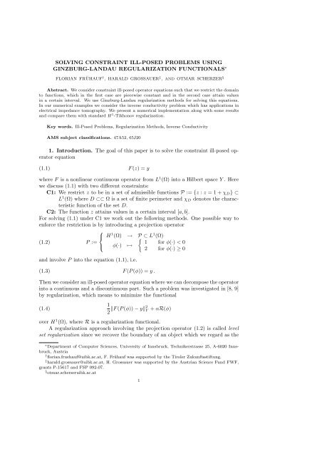
two squares constant “8” ramp “8” 

Fig. 4.1. The three conductivities which should be reconstructed. 

4. Results and Discussion. 

4.1. Examples for C1. In our experiments we take random initial data for real 

GL regularization, such that 1 ≤ z 0 (x) ≤ 2 for all x ∈ Ω. For this choice the initial 

values lie between the two minima of the potential W . We used a signed distance 

function centered in Ω as initial condition such that P ɛ (φ 0 )| ∂Ω = 1 and that P ɛ(φ ′ 0 ) > 0 

for some x ∈ Ω for the Tikhonov regularization. 

The conductivities which we want to reconstruct are plotted in figure 4.1 left, 

resp., middle. In figure 4.2, resp., 4.3 we show results obtained by using different regularizers 

for reconstructing. For the real GL regularizer we directly plot the solution 

z, whereas for the Tikhonov we plot the projection P ɛ (φ). Note that the resolution 

in figure 4.1 is finer than in the other figures. 

In the first experiment we want to reconstruct two squares located at opposite 

corners of Ω. For both regularizers a spurious signal remains in the center of Ω for 

many iterations. The reason for this phenomenon is that the influence of the boundary 

values spreads slowly into the interior. After the spurious signal has vanished higher 

values remain only in the locations of the squares. The shape of the two squares is better 

recognized with the real GL regularization, therefor with the Tikhonov regularizer 

the boundaries are sharper. 

In the second experiment a nonconvex inclusion should be reconstructed. We 

derive nearly the same effects for both regularizers as in the previous example. Again 

good reconstructions are achieved by the Tikhonov and the real GL regularization 

but the concavity on the right side is lost by the Tikhonov regularization. 

4.2. Examples for C2. For C2 we take initial data as follows: 

1. Tikhonov: z 0 (x) = 1 for all x ∈ Ω 

2. complex GL: R(v 0 (x)) = 1 and I(v 0 (x)) = 0 for all x ∈ Ω 

In the experiment we want to reconstruct the same “8”-shaped inclusion as for C1, but 

now we have a slope in the conductivity, cf. the right picture in figure 4.1. Note that 

this conductivity is not in H 1 (Ω) but the minimizers of the functionals necessarily are 

in H 1 (Ω). 

The results are plotted in figure 4.4. The Tikhonov regularization reconstructs 

the maximum values better, but there is a distinctive minimum of the values in the 

middle of the “8”. The slope of the conductivity is reconstructed by the complex GL 

method. Furthermore the reconstruction of the surrounding medium is better by the 

complex GL regularization. 

Now we consider the same example, where we add 3 % gaussian noise to the 

data. The reconstructions are shown in figure 4.5. Again the maximum values in the 

object are found better by the Tikhonov regularizer. But the slope is not recognized


Tikhonov, α = 0.06 

0 

2 

0 

2 

0 

2 

0.1 

1.9 

0.1 

1.9 

0.1 

1.9 

0.2 

1.8 

0.2 

1.8 

0.2 

1.8 

0.3 

1.7 

0.3 

1.7 

0.3 

1.7 

0.4 

1.6 

0.4 

1.6 

0.4 

1.6 

0.5 

1.5 

0.5 

1.5 

0.5 

1.5 

0.6 

1.4 

0.6 

1.4 

0.6 

1.4 

0.7 

1.3 

0.7 

1.3 

0.7 

1.3 

0.8 

1.2 

0.8 

1.2 

0.8 

1.2 

0.9 

1.1 

0.9 

1.1 

0.9 

1.1 

1 

0 0.2 0.4 0.6 0.8 1 

1 

1 

0 0.2 0.4 0.6 0.8 1 

1 

1 

0 0.2 0.4 0.6 0.8 1 

1 

after 50 iterations after 400 iterations after 2000 iterations 

Real Ginzburg-Landau, α = 10 −6 

0 

2 

0 

2 

0 

2 

0.1 

1.9 

0.1 

1.9 

0.1 

1.9 

0.2 

1.8 

0.2 

1.8 

0.2 

1.8 

0.3 

1.7 

0.3 

1.7 

0.3 

1.7 

0.4 

1.6 

0.4 

1.6 

0.4 

1.6 

0.5 

1.5 

0.5 

1.5 

0.5 

1.5 

0.6 

1.4 

0.6 

1.4 

0.6 

1.4 

0.7 

1.3 

0.7 

1.3 

0.7 

1.3 

0.8 

1.2 

0.8 

1.2 

0.8 

1.2 

0.9 

1.1 

0.9 

1.1 

0.9 

1.1 

1 

0 0.2 0.4 0.6 0.8 1 

1 

1 

0 0.2 0.4 0.6 0.8 1 

1 

1 

0 0.2 0.4 0.6 0.8 1 

1 

after 100 iterations after 1000 iterations after 3400 iterations 

Fig. 4.2. Course of evolution for the regularizers of C1 

Tikhonov 

Real Ginzburg-Landau 

0 

2 

0 

2 

0.1 

1.9 

0.1 

1.9 

0.2 

1.8 

0.2 

1.8 

0.3 

1.7 

0.3 

1.7 

0.4 

1.6 

0.4 

1.6 

0.5 

1.5 

0.5 

1.5 

0.6 

1.4 

0.6 

1.4 

0.7 

1.3 

0.7 

1.3 

0.8 

1.2 

0.8 

1.2 

0.9 

1.1 

0.9 

1.1 

1 

0 0.2 0.4 0.6 0.8 1 

1 

1 

0 0.2 0.4 0.6 0.8 1 

1 

α = 0.05, 4500 iterations 

α = 1 · 10 −6 , 1500 iterations 

Fig. 4.3. Stationary solutions of the regularizes of C1. 

satisfactory as well as the surrounding medium. The reconstruction with the complex 

GL regularizer of the surrounding medium is quite good. The constant slope of the 

conductivity in the object is found, but the values are not correct. 

REFERENCES 

[1] L. Ambrosio and N. Dancer. Calculus of Variations and Partial Differential Equations. Springer 

Verlag, 2000. 

[2] F. Bethuel, H. Brezis, and F. Helein. Ginzburg-Landau Vortices, volume 13 of Progress in 

Nonlinear Differential Equations and Their Applications. Birkhaeuser, 1994. 

[3] R.M. Brown and G. Uhlmann. Uniqueness in inverse conductivity problem for nonsmooth 

conductivities in two dimensions. Commun. Part. Diff. Equations, 22:1009–1027, 1997. 

[4] M. Burger. A level set method for inverse problems. Inverse Problems, 17:1327–1355, 2001. 

[5] T. Chan, J. Shen, and L. Vese. Variational pde models in image processing. Notices Amer. 

Math. Soc., 50:14–26, 2003. 

[6] S. Chen, B. Merriman, S. Osher, and P. Smereka. A simple level set method for solving stefan 

problems. J. Comput. Phys., 135:8–29, 1997. 

[7] H.W. Engl, M. Hanke, and A. Neubauer. Regularization of Inverse Problems. Kluwer Academic


Tikhonov 

Complex Ginzburg-Landau 

0 

0 

0.1 

1.7 

0.1 

1.6 

0.2 

1.6 

0.2 

0.3 

1.5 

0.3 

1.5 

0.4 

1.4 

0.4 

1.4 

0.5 

0.6 

1.3 

0.5 

0.6 

1.3 

0.7 

1.2 

0.7 

1.2 

0.8 

1.1 

0.8 

1.1 

0.9 

1 

0 0.2 0.4 0.6 0.8 1 

1 

0.9 

1 

0 0.2 0.4 0.6 0.8 1 

1 

1.7 

1.6 

1.8 

1.6 

1.8 

1.7 

1.7 

1.5 

1.6 

1.5 

1.6 

1.5 

1.4 

1.5 

1.4 

1.4 

1.4 

1.3 

1.3 

1.3 

1.3 

1.2 

1.2 

1.1 

1.2 

1.1 

1.2 

1 

0.9 

30 

20 

10 

10 

20 

30 

1.1 

1 

1 

0.9 

30 

20 

10 

10 

20 

30 

1.1 

1 

0 


0 

0 

α = 5 · 10 −6 , 1500 iterations 

0 

Fig. 4.4. Stationary solutions of both regularizes for C2. Note that the results are differently 

scaled. 

0 

Tikhonov 

0 

Complex Ginzburg-Landau 

0.1 

2 

0.1 

1.7 

0.2 

1.8 

0.2 

1.6 

0.3 

1.6 

0.3 

1.5 

0.4 

0.4 

0.5 

1.4 

0.5 

1.4 

0.6 

1.2 

0.6 

1.3 

0.7 

0.7 

1.2 

0.8 

1 

0.8 

1.1 

0.9 

0.8 

0.9 

1 

0 0.1 0.2 0.3 0.4 0.5 0.6 0.7 0.8 0.9 1 

1 

0 0.1 0.2 0.3 0.4 0.5 0.6 0.7 0.8 0.9 1 

1 

2 

1.7 

2.2 

2 

1.8 

1.8 

1.7 

1.6 

1.8 

1.6 

1.4 

1.2 

1 

0.8 

0.6 

1 

0.8 

1 

0.6 

0.8 

0.4 

0.6 

0.4 

0.2 

0.2 

0 0 


1.6 

1.4 

1.2 

1 

0.8 

1.6 

1.5 

1.5 

1.4 

1.4 

1.3 

1.2 

1.3 

1.1 

1 

1.2 

0.9 

1 

0.8 

1 

1.1 

0.6 

0.8 

0.4 

0.6 

0.4 

0.2 

1 

0.2 

0 0 

α = 6.3 · 10 −6 , 2500 iterations 

Fig. 4.5. Stationary solutions of both regularizes for C2 with noise. Note that the results are 

differently scaled.


Publishers, Dordrecht, 1996. 

[8] F. Fruehauf, O. Scherzer, and A. Leitao. Analysis of regularization methods for the solution 

of ill-posed problems involving discontinuous operations. SIAM Journal on Numerical 

Analysis, accepted for publication 2005. 

[9] R. Griesmaier. A level set method for the solution of the inverse conductivity problem and 

several distance measures as error criterion for inverse problems. Master’s thesis, Leopold 

Franzens University Innsbruck, Austria, 2004. 

[10] H. Grossauer and O. Scherzer. Using the complex ginzburg-landau equation for digital inpainting 

in 2d and 3d. Scale Space Methods in Computer Vision, pages 225–236, 2003. 

[11] M. Ipsen and P. Sorensen. Wavelength instabilities in a slow mode coupled complex ginzburglandau 

equation. Physical Review Letters, 84(11):2389, 2000. 

[12] V. Isakov. Inverse Problems for Partial Differential Equations, volume 127 of Applied Mathematical 

Sciences. Springer, 1998. 

[13] L. Landau and V. Ginzburg. On theory of superconductivity. Journal of Experimental and 

Theoretical Physics (USSR), 20:1064, 1950. 

[14] R. Stainko M. Burger. Phase-field relaxation of topology optimization with local stress constraints. 

Submitted to: SIAM Journal On Control and Optimization, submitted 2005. 

[15] E. de Wit M. van Hecke and W. van Saarloos. Coherent and incoherent drifting pusle dynamics 

in a complex ginzburg-landau equation. Physical Review Letters, 75(21):3830, 1995. 

[16] B. Merriman, J. Bence, and S. Osher. Motion of multiple functions: a level set approach. J. 

Comput. Phys., 112:334–363, 1994. 

[17] V.A. Morozov. Methods for Solving Incorrectly Posed Problems. Springer Verlag, New York, 

Berlin, Heidelberg, 1984. 

[18] V.A. Morozov. Regularization Methods for Ill-Posed Problems. CRC Press, Boca Raton, 1993. 

[19] S. Osher and J.A. Sethian. Fronts propagating with curvature-dependent speed: Algorithms 

based on Hamilton-Jacobi formulations. J. Comput. Phys., 79:12–49, 1998. 

[20] F. Santosa. A level set approach for inverse problems involving obstacles. ESAIM Contrôle 

Optim. Calc. Var., 1:17–33 (electronic), 1995/96. 

[21] G. Huber T. Bohr and E. Ott. The structur of spiral-domain patterns and shocks in the 2d 

complex ginzburg-landau equation. Physica D, 106:95–112, 1997. 

[22] H.-K. Zhao, T. Chan, B. Merriman, and S. Osher. A variational level set approach to multiphase 

motion. J. Comput. Phys., 127:179–195, 1996.

Solving constrained ill-posed problems using Ginzburg-Landau ...

Create successful ePaper yourself

Delete template?

Save as template?