Combined evolution of level sets and b-spline curves for imaging

Forschungsschwerpunkt S92
Industrial Geometry
http://www.ig.jku.at
INDUSTRIAL
GEOMETRY
Computer Aided Geometric Design
Computer Vision
FSP Report No. 41
Combined evolution of level sets and
B-spline curves for imaging
M. Fuchs, B. Jüttler, O. Scherzer and H.
Yang
January 2007

Abstract We propose the evolution of curves in direction
of their unit normal using a combined implicit and
explicit spline representation according to a given velocity
field. In the implicit case we evolve a level set
function for segmentation and geometry reconstruction
in 2D images. The level set approach allows for topological
changes of the evolving curves. The evolution of the
explicit B-spline curve is driven by the Mumford-Shah
functional.
We are mainly concerned with the segmentation of
images using active contours. To get satisfactory results
from the implicit evolution the optimal stopping time
and the correct level of the evolving function has to
be estimated. We overcome this problem by using the
combined evolution.
As a second application we focus at controlling the
topology of the level set function used to detect geometries
via EIT. The concurrent evolution of spline curves
enables us to identify geometries of dimension 1 which
would be lost using only the level set approach.

Noname manuscript No.
2
(will be inserted by the editor)
M. Fuchs · B. Jüttler · O. Scherzer · H. Yang
Combined evolution of level sets and B-spline curves for
imaging
the date of receipt and acceptance should be inserted later
1 Introduction
Level set methods introduced in [21] are widely used
in imaging to reconstruct geometries [6,7,9,11,10,12].
They automatically handle complex topologies, i.e. we
can detect and represent objects consisting of different
components by only one level set function. Also multiply
connected sets can be reconstructed. On the other
hand, since the geometry is implicitly hidden in the
graph of the level set function, one does not have direct
control over the geometry represented by the zero level
set. The additional evolution of curves driven by the
speed function adds the advantages of an explicit representation
to those of the level set evolution. We focus
on the application of this approach to the segmentation
of 2D gray-scale images. Secondly we suggest a way to
use the additional information provided by the spline
evolution to handle the correct detection of perfectly
insulating cracks in the EIT problem.
1.1 Image Segmentation
Several approaches to image segmentation have been
developed. One of them is the reconstruction of the
boundary of an object by detecting closed curves of high
gradients in the image. This is for instance described in
[15]. There the authors propose to minimize an energy
functional with respect to admissible splines such that
the minimizing splines optimally adapt to edges in the
M. Fuchs and O. Scherzer
Leopold-Franzens-Universität, Department of Computer Science,
Innsbruck, Austria
E-mail: matz.fuchs@uibk.ac.at
E-mail: otmar.scherzer@uibk.ac.at
B. Jüttler and H. Yang
Johannes-Kepler-Universität, Institute of Applied Geometry,
Linz, Austria,
E-mail: bert.juettler@jku.at
E-mail: yang.huaiping@jku.at
image, i.e. 1-dimensional features with high image gradients.
One possibility to obtain such a minimizer is to
evolve a closed curve from either outside or inside an
object towards the object boundaries. The speed of the
evolution is determined by the image gradients and
should be zero at the boundary. In this approach of
active contours the following issues have to be taken
care of:
– In regions, where no high image gradients occur, the
speed of the evolution has to be kept above a certain
level to provide convergence of the method. Noise in
the image, should not stop the evolution.
– The evolution should stop at the boundaries of the
object. The difficulty here is to correctly identify an
image region of high variation as a boundary. As
mentioned before, image noise can result in locally
high gradients. Thus, the shape of the moving contour
in the region in question has to be taken into
account as well as the absolute value of the gradient.
In other words, the evolving curve should not
get stuck at unwanted artifacts but, on the other
side, must not cross the object boundary.
– The regularity of the active contour has to be maintained.
If we require the curvature of the contour
to be bounded, it cannot stop at arbitrarily small
artifacts anymore. Secondly, even if we were able to
capture the exact boundary of an object, it may be
desired to further smooth the contour.
– Also the actual representation of the active contour
is of interest. In level set implementations the curve
will be the zero level set of a function discretized
at pixel level. For applications it can be crucial to
have a spline representation of the contour at hand,
which allows for easy corrections and adaptations in
a manual post-processing step. Secondly information
about the actual shape of the segmented object can
be acquired from a parametric representation more
easily. A simple example is the number of components
of the segmentation which is directly accessi-

3
ble by simply counting the number of evolving spline
curves.
A level set implementation of active contours was
proposed in [6] and extended in [7]. In the latter paper
the authors propose to evolve a level set function on R 2
according to
3
2
1
0
-1
5
4
3
2
1
u(0) = u 0 ,
∂u
( ( ∇u
) )
∂τ = |∇u|g(I σ) ∇ · + γ
|∇u|
+ ∇g(I σ ) · ∇u ,
(1.1)
-2
-1,5
-1
-0,5 0
x~
0,5
1
1,5
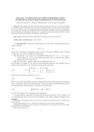
Fig. 1 Force function (green) for the Heaviside function
(red). We chose σ = .4 and η = 10. The balloon force is
γ = 1 (left) and γ = 5 (right).
0
-1
-1,5
-1
-0,5
0
x~
0,5
1
1,5
where g : R → R is a the so-called edge-detector, i.e.
a non-increasing, positive and differentiable function,
converging to 0 as its argument tends to infinity. We
denote the function defined by g(I σ )(x) = g ( |∇I σ (x)| )
for x ∈ R 2 as g(I σ ), where I σ is the image I : R 2 → R
after convolution with the Gaussian kernel determined
by σ. In accordance with [7] we call the parameter γ > 0
the balloon force. It is added to the curvature of u in
the first term of (1.1). This ensures that the level sets
move even in case their curvature is 0.
Assuming sufficient regularity on I and u 0 the authors
prove that a solution in the sense of viscosity solutions
of this equation exists. Considering objects with
boundaries {x ∈ R 2 : g(I)(x) = 0} they further show
that all level sets of u 0 , which initially enclose the object,
converge to the boundary of the object with respect
to the Hausdorff distance.
Because of the level set approach, this evolution automatically
adapts to topology changes. There exist numerous
implementations of this PDE. In the original paper
[7], the authors used finite differences both in time
and space. Kühne et al. [17] proposed the so-called AOS
scheme for efficient implementation. Yang et al. [22] use
a T-Spline representation of the level set function. For
the results in this paper we discretized the space domain
with finite elements and used finite differences in
time.
All of the above mentioned implementations share
the following parameters:
– The balloon force γ.
– The initial level set function u 0 .
– The edge detector g. Regardless of the exact function
chosen for as edge detector, there will be a parameter
η controlling how sensitive the edge detector
is with respect to gradients. Common choices for g
are
g(t) = exp(ηt 2 ) or g(t) =
1
1 + ηt 2 .
Often semi-implicit schemes additionally require to regularize
the term |∇u| to avoid singularities. The regularization
also influences the results of these methods.
The influence of γ is illustrated by the following example.
The explicit evolution of the zero level set of
(1.1) is given by
∂C
∂τ · n = g(I σ)(γ + κ) − ( ∇g(I σ ) · n ) ,
where C denotes the evolving the curve, κ its curvature
and n its normal. For simplicity we focus on the
1-dimensional case and assume κ = 0. We then see that
the explicit curve is driven by the force γg(I σ )−|g ′ (I σ )|.
Consider the image I = H, the Heaviside function. In
Figure 1 we plotted the attraction force in this case for
different parameters γ and η. Imagine the active contour
arriving from the left. In the regions where the
force function is positive the contour is pushed towards
the edge (at 0). The negative force pulls the contour
back again and traps it at 0. If the region of negative
force is small, it is likely that the curve crosses the edge
due to numerical inaccuracies.
When using the above method we often observe that
already detected parts of the boundary in the outer regions
of the image vanish before the central image regions
are segmented. This is illustrated in the upper
three images in Figure 2. At no time τ the complete
boundary of the object is correctly detected, since the
active contour crosses the boundary in the outer regions
at an early stage of the evolution.
There are two main reasons for this phenomenon.
First, the active contour crosses the boundary if the
gradient at the edge is too small for the edge detector
to locally stop the evolution. This essentially means that
the user has to choose a high enough value for η to stop
the evolving curve at the “right” edge. In other words,
the choice of the parameter η determines the steepness
of the edges which will eventually be detected.
Secondly, the first term in the evolution equation
never degenerates completely and thus the level set function
increases due to the balloon force. Therefore, after
some time u is raised above the zero level and the
boundary of the object vanishes.
In Figure 2 the latter effect clearly dominates. Obviously
the information on the object boundary is still

4
2
1.5
1
0.5
0
−0.5
−1
0
20
40
60
10
20
30
40
50
60
n = 0
2
Fig. 3 Detection of a square with salt & pepper noise added:
solution of the evolution at τ = 1800 started from an initial
function u 0 (left) and from 5u 0 (right).
1.5
1
0.5
0
−0.5
−1
0
20
n = 5
−1
2
1.5
1
0.5
0
−0.5
0
20
n = 40
Fig. 2 Vanishing boundary at the outer regions of the image.
available at any time but can not be captured by the
zero level set.
This is visible first at the outer parts of the image
domain, where the initial function is close to 0. Note
that theoretically the problem does not exist, but it occurs
due to technical limitations in the implementation
of equation (1.1) and is amplified by large balloon forces
γ as it is explained in more detail in the following:
– To ensure that in each time step we solve a PDE
in divergence form, we have to divide equation (1.1)
by |∇u|. In numerical realizations this term has to
be regularized to avoid divisions by zero, i.e. we
substitute |∇u| by √ ∇u · ∇u + ε 2 for some small
ε > 0. We call this approximation of the gradient
ε-regularization. This modification implies that the
principal component of the evolution equation is always
positive, even if the level set function is flat. To
approximate the original equation, it is preferable to
choose ε as small as possible, but clearly this choice
is limited by numerical considerations.
– It is desirable to choose γ large for two reasons.
Firstly, higher values of γ give faster evolution speeds.
Secondly, Caselles et al. require γ to be large enough
40
40
60
60
10
10
20
20
30
30
40
40
50
50
60
60
to obtain the result concerning consistency of the active
contour method in [7].
Unfortunately the influence of the ε-regularization
is multiplied by the balloon force. Thus, one has to
balance evolution speed against the ε-regularization.
– A very steep initial function u 0 is robust against
the effect of vanishing boundaries. E.g. it is possible
to avoid the problems in Figure 2 by rescaling u 0 .
The drawback is that steep level set functions are
more sensitive to noise. This is illustrated in Figure
3. Again a compromise between sensitivity to noise
and global stability of the result has to be found.
All the above issues cause the level lines of the evolving
function u to move across the boundary of the object
we want to detect. If this happens, we can not extract a
reliable segmentation from the zero level set anymore.
Thus, we consider a method to extract the boundary information
from the level set function without sticking to
a specific level. We propose to evolve a B-Spline curve,
which splits according to the topology information provided
by the normal vectors of the level set function.
By combining the evolution of the active contour with a
Mumford-Shah type segmentation of the level set function
we inherently use the information of all level sets
in contrast to tracking only one. We go even further by
additionally using the derivative of the level set function
to extract information about the topology of the
target shape. The B-Spline representation can easily be
manually adapted during or after the evolution and allows
for precise control of the regularity of the resulting
contour.
1.2 Electrical Impedance Tomography
Electrical Impedance Tomography (EIT) is concerned
with the identification of inclusions in a conductor by
measuring the potentials induced by current fluxes on
the boundary. Assuming a planar conductor (i.e. the
2-dimensional case) and the special case of perfectly
isolating inclusions and constant conductivity on the
remaining region, it can be shown [14,2,16] that the
inclusions can be uniquely determined by at most two

5
measurements. This result holds for inclusions of dimension
2 and 1.
The actual identification of these inclusions by computational
means is an ill-posed inverse problem. Results
concerning the (in-)stability of the reconstruction
can be found in [14,1,3,5,4]. We will focus on a level
set implementation which is similar to [10,12]. This iterative
approach starts with a level set function such
that the zero level set corresponds to the initial guess
of the inclusion. The level set function evolves according
to the minimizing gradient flow of a regularization
functional. Thus, we have a level set evolution
u k+1 = u k − δ∇F(u k ),
where F is the regularization energy (corresponding to
the EIT problem) and ∇F its derivative with respect to
the level set function u. Then u k is supposed to converge
to a function ũ in the L 2 sense, such that {x ∈ Ω :
ũ(x) ≥ 0} is the isolating inclusion we seek.
Now assume that this inclusion is a crack, i.e. a
1-dimensional set. Then, it can not be characterized by
a level set function of class L 2 anymore and the above
method will fail. In other words, a level set method
which is known to detect inclusions in a conductor in
the L 2 -sense only, does not work for cracks anymore,
because 1-dimensional features will be lost with such a
method.
We propose to use a combined evolution in the iterative
computation of such level set functions. It might
allow us to detect the development of level sets of dimension
1 in advance and to cope with such cases. This
approach is very similar to the case of image segmentation
and is described in detail in Section 4.
2 The combined evolution
As in the introduction we assume a gray-scale image
I : R 2 → R and an initial level set function u 0 . Let
further u : [0, ∞[ × R 2 → R be a solution of (1.1) and
C j : [0, 1] → R 2 , 1 ≤ j ≤ k, simple Jordan curves,
which do not intersect each other (or lie within each
other). By I(C) and O(C) we denote the regions inside
and outside a Jordan curve C : [0, 1] → R 2 . We further
define
I(C 1 , . . . , C k ) = ⋃
1≤j≤k
O(C 1 , . . . , C k ) = ⋂
1≤j≤k
I(C j ) and
O(C j ).
A slightly modified version of the Mumford-Shah functional
[19,20], for k curves is given by
∫
(
I(C 1 , . . .,C k ) = α u1 − f ) 2
dx
I(C 1,...,C k )
+ α
+ β
∫
O(C 1,...,C k )
k∑
L 2 2(C j ),
j=1
where α, β > 0 and
∫
u 1 = avg f dx and u 2 = avg
Here
I(C 1,...,C k )
(
u2 − f ) 2
dx
∫
avg f dx := 1 ∫
f dx
A |A| A
∫
O(C 1,...,C k )
(2.1)
f dx.
is the average of a function f over a set A. The functional
(2.1) is also used in [11].
We want to minimize the above energy functional
by solving the variational problem I → min. Assume
that C 1 ′, . . . C′ k
are curves of minimal energy. Then the
function
u ′ = u 1 χ I(C1,...,C k ) + u 2 χ O(C1,...,C k )
is a piecewise constant function, which is discontinuous
along the boundaries of C j only and approximates u in
the L 2 sense.
Differentiation of I(C 1 , . . . , C k ) with respect to C j ,
1 ≤ j ≤ k, yields the following gradient descent:
∂C j
∂τ (τ) = −∇I( C j (τ) ) , 1 ≤ j ≤ k , (2.2)
where
−∇I ( C ) ( (u2
= α (C) − u ◦ C ) 2
− ( u 1 (C) − u ◦ C ) 2 ) |C ′ |n j
+ β|C ′ |C ′′ ,
(2.3)
for a curve C. Here ∇I is the derivative of the energy
functional I in (2.1) with respect to C. Although we
denote it by ∇I, it can not expressed as a matrix since
I is defined on an infinite-dimensional space.
Note that we include the derivative of C with respect
to the curve parameter t in ∇I(C). I.e. the directional
derivative of the functional I in C into the direction D
can be computed by simply integrating ∇I(C) · D over
the parameter interval [0, 1],
DI(C)(D) =
∫ 1
0
∇I(C)(t) · D(t)dt .

6
Assume k initial curves C1, 0 . . . , Ck 0 . Combining equations
(1.1) and (2.3) gives
u(0) = u 0 ,
C j (0) = Cj 0 , 1 ≤ j ≤ k ,
∂u
(
∂τ = |∇u|g(I σ) ∇ ·
∂C j
∂τ = −∇I( C j (τ) ) .
( ∇u
|∇u|
) )
+ γ + ∇g(I σ ) · ∇u ,
(2.4)
In the above equation u and C j and hence also n and
κ are functions of the time τ, i.e. u = u(τ), C j = C j (τ),
n = n(τ) and κ = κ(τ). Note that this system is decoupled
in the sense that the equations governing the
evolution of the C j , 1 ≤ j ≤ k depend on the first equation
(the evolution of u) but not the other way round.
In the following we motivate the use of this evolution
for segmentation. Theorem 1 shows that the level
set function of the above evolution converges to the indicator
function of the object which is to be detected. It is
based on the results in [7]. We will state all of the following
results for the case k = 1 to simplify the notation.
The generalization to the case k > 1 is straightforward.
Theorem 1 (Caselles et al.) Assume that the edge
detector g(I σ ) : R 2 → [0, ∞[ satisfies g(I σ ) ≥ 0 and
sup |∇g 1/2 (x)| < ∞ and sup |D 2 g(x)| < ∞ .
x∈ R 2 x∈ R 2
Let further be Ĉ : [0, 1] → R 2 a simple C 2 -Jordan
curve, which parametrizes
{x ∈ R 2 : g(I)(x) = 0} = image(Ĉ),
and is such that ∇g(I) = 0 on image(Ĉ).
We require the initial function u 0 : R 2 → R, u 0 ≥ 0,
to be of class u 0 ∈ C 2 ( R 2 ). Further u 0 should be 1 on
a neighborhood of I(Ĉ) and 0 outside a bounded set
Ω ⊆ R 2 .
Define for 0 < h ≤ 1
C(τ, h) = ∂{x ∈ R 2 : u(τ, x) ≥ h} .
Then there exists a unique viscosity solution u(τ, x) of
(1.1) satisfying
inf u0 (x) ≤ u(τ, x) ≤ sup u 0 (x) for τ ≥ 0.
x∈ R 2 x∈ R 2
If γ is large enough then the following results hold: For
every 0 < h ≤ 1
lim C(τ, h) = Ĉ (2.5)
τ →∞
with respect to the Hausdorff distance, and
lim u(τ) = χ
τ →∞ I(Ĉ) in the L 2 -sense. (2.6)
Proof The result concerning existence and uniqueness
and (2.5) has been proved in [7].
Thus, it remains to prove (2.6). In the proof of Theorem
5 in [7] and Theorem 4 in [8] the authors obtain
the result (2.5) by showing that for ε > 0 and 0 < h ≤ 1
there exists τ 0 > 0 such that for τ ≥ τ 0 the level set
function is bounded by h on the outside of the ε-offset
of Ĉ, i.e.
sup { u(τ, x) : x ∈ R 2 , x ∉ I(Ĉ) ε, τ > τ 0} < h .
Here I(Ĉ) ε = I(Ĉ) + B ε(0). Secondly, u(τ, x) = 0 on
R 2 \ Ω.
Now assume ε > 0 and let τ 0 be as above for the
special case h = 1 − ε. Then
∫
∫ ∫
(
χI( Ĉ) − u(τ)) 2
dx ≤ ε 2 + 1 dx
R 2 Ω\I(Ĉ)ε I(Ĉ)ε\I(Ĉ)
≤ |Ω|ε 2 dx + |Ĉ + B ε(0)| ,
since u(τ) = 1 on I(Ĉ) for all τ ≥ 0. Here | · | denotes
the 2-dimensional Lebesgue measure of a set. Note that
the above convergence holds also in L p for 1 ≤ p < ∞.
⊓⊔
Theorem 1 states that for τ → ∞ the function u(τ)
converges to the indicator function of the object. It is
difficult to prove analytically, but intuitively evident
that the curve C approximates the boundary of the object
as well. The parameter α controls the smoothness
of the boundary C during the evolution. This allows for
effective capturing of objects with noisy boundary.
In general the viscosity solution does not have to
be differentiable but is just continuous. However, we
can still compute the generalized gradient ∇u in every
is the unit
normal of the level sets of u. Thus, in the view of Theorem
1, we can at least formally expect that
point. If |∇u| is finite and positive then ∇u
|∇u|
∇u(τ)
≈ n(τ) for τ → ∞ . (2.7)
|∇u(τ)|
We will use this observation to correctly adapt the topology
of the moving spline curves C j during the evolution.
If during the evolution two separate parts of C j get close
to each other and the relation (2.7) does not hold in this
area, we have to split the curve into two curves. This is
illustrated in Figure 4 and explained in more detail in
the next section.
3 Implementation
To solve (2.4) numerically we model u(τ) using bilinear
finite elements on a regular pixel-sized grid. The
evolving spline curve C(τ) is implemented with periodic
cubic B-splines.

7
Multiplying the above equation by a test function ϕ m ,
1 ≤ m ≤ N, and inserting the base function representation
of u and integrating it over Ω yields the discretization
in space and time,
Fig. 4 Adaptation of the topology of the evolving spline
curve (red) to the topology prescribed by the level set function
(green). On the left the normals of the spline curve and
the gradients of the level set function are orthogonal to each
other. This indicates that the spline curve has to be splitted.
On the right the two segments of the spline curve are very
close to each other but there topology conforms with the level
set function. No splitting is performed.
The numerical solution of (2.4) is performed in three
steps. At a given time τ ≥ 0 we compute an approximate
solution u(τ + δ) by solving the semi-implicit
system of equations derived from the FE-formulation.
In the second step we evolve C(τ) to τ + δ using explicit
steps in time. In the last step we detect topology
changes by comparing the gradients of the level set function
to the curve normals as explained in Figure 4. In
case the topology of the curve does not correspond to
the level set topology (which we assume to be correct),
we adapt the curve to the level-set function by splitting
into more components. Finally we proceed with computing
the next step of the semi-implicit evolution.
3.1 Level set evolution
For τ ≥ 0 and the time step δ > 0 the semi-implicit
time discretization of (1.1) on Ω reads as
u(τ + δ) − u(τ)
δ
(
∇u(t + τ)
)
= |∇u(t)|∇ · g(I σ )
|∇u(t)|
+ γ|∇u(t + τ)|g(I σ ).
We cover the rectangular image domain Ω with square
elements with corners at the centers of the image pixels.
On this grid we define bilinear basis functions
(ϕ n ) 1≤n≤N . Then we identify
u 0 (x) =
u(τ, x) =
N∑
u 0 nϕ n (x) and
n=1
N∑
u n (τ)ϕ n (x) for x ∈ Ω .
n=1
N∑
n=1
where
∫
u n (τ + δ)
Ω
a ( ∇u(τ, x) ) ϕ n (x)ϕ m (x)dx
∫
+ b ( x, ∇u(τ, x) ) ∇ϕ n (x)∇ϕ m (x)dx
Ω
∫
= c ( x, u(τ, x), ∇u(τ, x) ) ϕ m (x), (3.1)
Ω
a(ξ) = 1
|ξ| ,
b(x, ξ) = δg(I σ)(x)
,
|ξ|
c(x, p, ξ) = p
|ξ| + δγg(I σ)(x).
Assuming that u(τ) is known this is a system of linear
equations for u n (τ + δ), 1 ≤ n ≤ N.
To avoid singular coefficients we regularize |ξ| in a,
b and c by replacing it by Ψ ε (|ξ|). In our case we chose
Ψ ε (|ξ|) = √ |ξ| 2 + ε 2 . Finally we get u(τ +δ) by approximating
N∑
u(τ + δ) ≈ u n (τ + δ)ϕ n ,
n=1
where the u n (τ + δ), 1 ≤ n ≤ N, are the solutions of
equation (3.1) with the ε-regularization in the coefficients
mentioned above.
3.2 Spline evolution
Let C 1 p([0, 1], Ω) be the space of continuously differentiable
and periodic curves equipped with the L 2 -norm.
Assume the basis of periodic cubic B-Splines
ψ = (ψ k : [0, 1] → R ) 1≤k≤K , ψ k ∈ C 1 p with uniformly
distributed knots. Let further C(τ) be a B-Spline curve
based on (ψ k ) 1≤k≤K . Thus, for τ ≥ 0 we have
C ( p(τ) ) =
K∑
p k (τ)ψ k
k=1
where p(τ) = ( p 1 (τ), . . . , p K (τ) ) , and
p k = (p 1 k, p 2 k) : [0, ∞[→ R 2 , 1 ≤ k ≤ K ,
are the time-dependent spline control points. That is,
we reinterpret the symbol C as a function which maps
the spline control points p to a parametrized curve:
C : ( R 2 ) K → C 1 p([0, 1], R 2 ). (3.2)
We denote the derivative of C(p) with respect to p as
DC(p) and its adjoint as DC(p) ∗ . That means DC(p)

8
linearly maps a v ∈ ( R 2 ) K to DC(p)(v) ∈ C 1 p([0, 1], R 2 ).
Transforming the gradient descent in (2.3) to the evolution
of the corresponding spline control points yields
DC(p) ∗ ◦ DC(p) ◦ ∂p
∂τ = −∇I( C(p) ) ◦ DC(p),
and consequently
∂p
∂τ = −∇I( C(p) ) ◦ DC(p) ◦ ( (DC(p) ∗ ◦ DC(p) ) −1
.
Let A be the matrix defined by
A ij =
∫ 1
0
ψ i (t)ψ j (t)dt ,
(3.3)
and B = A −1 . Then computation yields the explicit
evolution of the i-th component of the k-th spline coefficient
(i = 1, 2 and 1 ≤ k ≤ K):
∂p i K k
∂τ = − ∑
∫
j=1
C(p)
(
∇I
(
C(p)
)
(t)
) iψ j (t)B jk dt . (3.4)
We implemented (3.4) using explicit steps in time, i.e.
we compute
p i (τ + δ ′ ) = p i (τ) + δ ′(∫ Φ ( C(p) ) )
i
ψ k ds
C(p)
◦ ( DC(p) ∗ ◦ DC(p) ) −1
.
In our implementation we set δ ′ = δ/50 for all examples.
3.3 Topology Adaptation
During the evolution of C(τ) we adapt the spline curve
to topology changes of level sets of u. After each step
of the implicit evolution we look for self-intersections of
every spline curve. As stated in the previous section we
assume that the gradients of the level set function u(τ)
reflect the topology of the level sets. Thus, in case a
self-intersection occurs, we check if ∇u(τ)/|∇u(τ)| and
the normals of the curve n(τ) locally coincide. If not, we
split the curve into two and proceed with the evolution
of k + 1 curves.
4 Electrical Impedance Tomography (EIT)
conductivity
Assume a 2-dimensional, simply connected conductor
Ω with smooth boundary, a current flux f ∈ L 2 (∂Ω),
and a closed curve Ĉ in Ω. Again denote the area inside
and outside of Ĉ as I(Ĉ) and O(Ĉ), respectively. If the
is constantly 1 on O(Ĉ) and 0 on I(Ĉ), then
the electrical potential satisfies the following equation:
∆ϕ = 0 on O(Ĉ),
∂ϕ
= f
∂n
on ∂Ω ,
∂ϕ
= 0
∂n
on Ĉ.
(4.1)
If the boundary Ĉ is smooth, this problem has a
unique weak solution in W 1,2( O(Ĉ)) (e.g. [18, Section
3.6.]) We are concerned with the problem of obtaining
the geometry of the inclusion from measurements of the
electrical potential on the outside of the conductor, i.e.
from ϕ|Ĉ. In [2] (see also [16]) the authors have shown
that two measurements of ϕ|Ĉ (corresponding to two
different current fluxes) are sufficient to reconstruct the
inclusions.
Let u ∈ L 2 (Ω) and define the zero level set
Ω u := {x ∈ Ω : u(x) ≤ 0}.
We introduce the Neumann-to-Dirichlet operator
G u : L 2 (∂Ω) → L 2 (∂Ω), which maps a current flux f
to the trace of the solution of (4.1), where Ĉ is replaced
by ∂Ω u and O(Ĉ) by Ω u. Now consider current fluxes
f i ∈ L 2 (∂Ω) and electrical potentials g i ∈ L 2 (∂Ω) on
the boundary of the conductor. We define the following
Tychonov-type regularization functional (cf. [13])
F γ (u) = 1 2
N∑
‖G u (f i ) − g i ‖ 2 L 2 (∂Ω) + γ 2 ‖u‖2 L 2 (Ω) . (4.2)
i=1
Setting ϕ i := G u (f i ), the formal derivative of F γ with
respect to ϕ is
∇F γ (u) = −
N∑
i=1
∂ 2 ϕ i
∂n 2
v i
|∇u| δ u + γu , (4.3)
where v i , 1 ≤ i ≤ N, are the solutions of
∆v i = − ( ϕ i − g i
)
on Ω \ Ω u ,
∂v i
∂n = 0 on ∂Ω ∪ ∂Ω u ,
(4.4)
and δ u is the gradient of the indicator function of Ω u
in the distributional sense, i.e. the 1-dimensional Dirac
delta function along the zero level line of u. We propose
the gradient flow
∂u( ) ( )
u(τ) = −∇Fγ u(τ)
∂τ
(4.5)
to minimize (4.2). For numerical implementations it is
convenient to ε-regularize |∇u| in the denominator in
(4.3) and to approximate δ u by a smooth kernel δ ε u.

9
Again we propose a combined evolution of the level
set functions and spline curves C 1 , . . . , C k similar to
(2.4):
∂u
∂τ = −∇F ( )
γ u(τ) , u(0) = u 0 ,
∂C j
∂τ = −∇I( C j (τ) ) (4.6)
, C j (0) = Cj 0 ,
where for a curve C
−∇I ( C ) ( (u2
= α (C) − u ◦ C ) 2
− ( u 1 (C) − u ◦ C ) 2 ) |C ′ |n j
+ β|C ′ |C ′′ .
As in Section 2 we denote by u 1 (C) and u 2 (C) the
average value of the level set function u inside and outside
the curve C, respectively. In addition to handling
changes of the topology of the evolving curves (as in Section
3.3) the shape characteristics of the spline curves
can be tracked. In case the inclusion Γ is a crack, i.e. a
set of dimension 1, we can not detect it by the level set
function u in the L 2 sense anymore. The development
of very thin curves C in the evolution (4.6) indicates
such a case in advance.
Note that we are not able to prove that the level
set function u converges to the indicator function of an
inclusion Γ as we did in Theorem 1 for the case of image
segmentation.
5 Results
In this section we present the numerical results for the
combined evolution (2.4). In all test cases, except the
ones shown in Figures 9 and 10, we chose α = 10,
β = 0.1 (with the exception of β = 3 in the example
in Figure 7) and the balloon force γ = 0.2. The time
step δ of the semi-implicit FE step varies from δ = 20
to δ = 100. The number of steps of the implicit evolution
is denoted by n in the illustrations, the number of
steps of the explicit (curve) evolution is 50n. With the
exception of the first example we chose ε = 10 −3 in the
regularization of |∇u| −1 . The edge detection parameter
is η = 100. In all the images the red curves are the
spline curves corresponding to the C j (τ) in (2.4). The
zero level set of the function u(τ) is painted in green.
In Figure 5 we computed the combined evolution
(2.4) for the cross presented in the introduction. To illustrate
the influence of the regularization of |∇u| −1 we
chose ε = 10 −2 of one order larger. This example shows
the stability of the spline curve compared to the zero
level set of the geodesic active contour.
In Figure 6 we added salt & pepper noise to an underlying
binary image. The spline curve adapts itself
to the components of the object and attains a stable
steady state. Figure 7 illustrates the regularizing effect
Implicit evolution
≈ 95 seconds
Table 1 Computation times.
Combined evolution
≈ 18 seconds
of higher values for β. It also demonstrates that we detect
high gradients and not areas of similar contrast. In
Figure 8 we can observe the adaptation of the spline
curve to the topology of the object by using the gradients
of the level set function.
For illustrative reasons we chose different values of
δ in the above examples, but the evolutions behave the
same, when setting δ = 100 and thus reducing the number
of steps required to obtain the final image to n = 8
and n = 10 in Figure 5 and Figure 8 respectively.
In the last example the choice of parameters is different
from above. We segmented cell clusters in DIC (Differential
Interference Contrast) images. First we evolved
the level set function without the spline curve and tried
to choose the parameters such that the segmentation
worked as well as possible (Figure 9). We then compared
this result to the combined evolution with different parameters
for the implicit part of the evolution (Figure
10). We observe that the results of both methods are
roughly the same (the first one being more precise on
the edges) but the combined evolution requires much
less steps to reach the final segmentation. Considering
the fact that the explicit evolution of the spline curves
is fast compared to the implicit evolution this results in
significantly lower computation times for the combined
evolution (Table 1). In other words, the added curve
evolution allows us to choose the parameters controlling
the level set evolution such that the evolution is
much faster than before without loosing sensitivity. In
addition, if we are mostly interested in the number of
cell clusters, we can get this information immediately
from the result of the combined evolution (simply by
counting the number or spline curves).
Acknowledgements This work has been supported by the
Austrian Science Foundation (FWF) Projects Y-123INF,
FSP9202-N12, FSP9203-N12 and FSP9207-N12. We thank
Jean-Paul Zolésio, INRIA, Sophia-Antipolis, France, for stimulating
discussion. Finally we want to express our gratitude
towards Heimo Wolinski, IMB-Graz, Karl-Franzens-Universität,
Graz, Austria, and Bettina Heise, FLLL, Linz-Hagenberg,
Austria, for the image data (Figures 9 and 10).
References
1. G. Alessandrini. Stability for the crack determination
problem. In L. Päivärinta and E. Somersalo, editors,
Inverse Problems in Mathematical Physics, volume 422
of LNP, pages 1–8, 1993.
2. G. Alessandrini and A. Diaz Valenzuela. Unique determination
of multiple cracks by two measurements. SIAM
J. Control Optim., 34:913–921, 1996.

10
n = 0 n = 5
3. Giovanni Alessandrini. Examples of instability of inverse
boundary-value problems. Inverse Problems, 13(4):887–
897, 1997.
4. Giovanni Alessandrini and Luca Rondi. Stable determination
of a crack in a planar inhomogeneous conductor.
Inverse Problems, 30(2):326–340, 1998.
5. Stéphane Andrieux, Amel Ben Abda, and Mohamed
Jaoua. On the inverse emergent plane crack problem.
Mathematical Methods in the Applied Sciences, 21:895–
906, 1998.
6. Vicent Caselles, Francine Catté, and Françoise Dibos. A
geometric model for active contours in image processing.
Numerische Mathematik, 66:1–31, 1993.
7. Vicent Caselles, Ron Kimmel, and Guillermo Sapiro.
Geodesic active contours. International Journal of Comn
= 0 n = 20
n = 20 n = 40
Fig. 5 Cross. ε = .01, δ = 20.
n = 50 n = 70
Fig. 7 Star-like object with large variation of the boundary.
β = 3, δ = 100.
n = 0
n = 0 n = 40
n = 20
n = 80 n = 120
Fig. 6 Multiple segments with salt & pepper noise. δ = 100.
n = 30
n = 40
Fig. 8 Similar objects of different topology. δ = 25.

11
n = 10 n = 80
n = 160 n = 240
Fig. 9 Detection of cell clusters (active contours).
δ = 10, ε = 0.001, γ = 0.05, η = 1000.
n = 0 n = 5
puter Vision, 22(1):61–79, 1997.
8. Vicent Caselles, Ron Kimmel, Guillermo Sapiro, and
Catalina Sbert. Minimal surfaces: A three dimensional
segmentation approach. Technical Report 973, Technion
EE Pub., 1995.
9. Vicent Caselles, Ron Kimmel, Guillermo Sapiro, and
Catalina Sbert. Minimal surfaces based object segmentation.
IEEE Transactions on Pattern Analysis and Machine
Intelligence, 19(4):394–398, 1997.
10. Tony F. Chan and Xue-Cheng Tai. Level set and total
variation regularization for elliptic inverse problems
with discontinuous coefficients. Journal of Computational
Physics, 193(1):40–66, 2004.
11. Tony F. Chan and Luminita A. Vese. Active contours
without edges. IEEE Transactions on Image Processing,
10(2):266–277, 2001.
12. Eric T. Chung, Tony F. Chan, and Xue-Cheng Tai. Electrical
impedance tomography using level set representation
and total variational regularization. Journal of Computational
Physics, 205(1):357–372, 2005.
13. Heinz W. Engl, Martin Hanke, and Andreas Neubauer.
Regularization of Inverse Problems, volume 375 of Mathematics
and Its Applications. Kluwer Academic Publishers,
Dordrecht Boston London, 2000.
14. Avner Friedman and Michael Vogelius. Determining
cracks by boundary measurements. Indiana Univ. Math.
J., 38:527–556, 1989.
15. M. Kass, A. Witkin, and D. Terzopoulos. Snakes active
contour models. International Journal of Computer Vision,
1(4):321–331, 1988.
16. Hyunseok Kim and Jin Keun Seo. Unique determination
of a collection of a finite number of cracks from two
boundary measurements. SIAM J. Math. Anal., 27:1336–
1340, 1996.
17. Gerald Kühne, Joachim Weickert, Markus Beier, and
Wolfgang Effelsberg. Fast implicit active contour models.
In Pattern Recognition : 24th DAGM Symposium,
Zurich, Switzerland, September 16-18, 2002. Proceedings,
volume 2449 of Lecture Notes in Computer Science,
pages 133–140, Berlin/Heidelberg, 2002. Springer.
18. Olga A. Ladyshenskaya and Nina N. Ural’tseva. Linear
and Quasilinear Elliptic Equations, volume 46 of Mathematics
in Science and Engineering. Academic Press,
New York and London, 1968.
19. D. Mumford and J. Shah. Boundary detection by minimizing
functionals. In Proc. IEEE Conf. Computer Vision
Pattern Recognition, pages 22–26, 1985.
20. D. Mumford and J. Shah. Optimal approximations by
piecewise smooth functions and associated variational
problems. Commun. Pure Appl. Math., 42(4):577–684,
1989.
21. S. Osher and J.A. Sethian. Fronts propagating
with curvature-dependent speed: Algorithms based on
hamilton–jacobi formulations. Journal of Computational
Physics, 79:12–49, 1988.
22. Huaiping Yang, Matthias Fuchs, Bert Jüttler, and Otmar
Scherzer. Evolution of t-spline level sets with distance
field constraints for geometry reconstruction and image
segmentation. In IEEE International Conference on
Shape Modeling and Applications 2006 (SMI’06), pages
247–252, Los Alamitos, CA, USA, 2006. IEEE Computer
Society.
n = 10 n = 15
Fig. 10 Detection of cell clusters (combined evolution).
δ = 100, ε = 1.0, γ = 0.5, η = 1000.