Combined evolution of level sets and b-spline curves for imaging
Combined evolution of level sets and b-spline curves for imaging
Combined evolution of level sets and b-spline curves for imaging

Create successful ePaper yourself
Turn your PDF publications into a flip-book with our unique Google optimized e-Paper software.
9<br />
Again we propose a combined <strong>evolution</strong> <strong>of</strong> the <strong>level</strong><br />
set functions <strong>and</strong> <strong>spline</strong> <strong>curves</strong> C 1 , . . . , C k similar to<br />
(2.4):<br />
∂u<br />
∂τ = −∇F ( )<br />
γ u(τ) , u(0) = u 0 ,<br />
∂C j<br />
∂τ = −∇I( C j (τ) ) (4.6)<br />
, C j (0) = Cj 0 ,<br />
where <strong>for</strong> a curve C<br />
−∇I ( C ) ( (u2<br />
= α (C) − u ◦ C ) 2<br />
− ( u 1 (C) − u ◦ C ) 2 ) |C ′ |n j<br />
+ β|C ′ |C ′′ .<br />
As in Section 2 we denote by u 1 (C) <strong>and</strong> u 2 (C) the<br />
average value <strong>of</strong> the <strong>level</strong> set function u inside <strong>and</strong> outside<br />
the curve C, respectively. In addition to h<strong>and</strong>ling<br />
changes <strong>of</strong> the topology <strong>of</strong> the evolving <strong>curves</strong> (as in Section<br />
3.3) the shape characteristics <strong>of</strong> the <strong>spline</strong> <strong>curves</strong><br />
can be tracked. In case the inclusion Γ is a crack, i.e. a<br />
set <strong>of</strong> dimension 1, we can not detect it by the <strong>level</strong> set<br />
function u in the L 2 sense anymore. The development<br />
<strong>of</strong> very thin <strong>curves</strong> C in the <strong>evolution</strong> (4.6) indicates<br />
such a case in advance.<br />
Note that we are not able to prove that the <strong>level</strong><br />
set function u converges to the indicator function <strong>of</strong> an<br />
inclusion Γ as we did in Theorem 1 <strong>for</strong> the case <strong>of</strong> image<br />
segmentation.<br />
5 Results<br />
In this section we present the numerical results <strong>for</strong> the<br />
combined <strong>evolution</strong> (2.4). In all test cases, except the<br />
ones shown in Figures 9 <strong>and</strong> 10, we chose α = 10,<br />
β = 0.1 (with the exception <strong>of</strong> β = 3 in the example<br />
in Figure 7) <strong>and</strong> the balloon <strong>for</strong>ce γ = 0.2. The time<br />
step δ <strong>of</strong> the semi-implicit FE step varies from δ = 20<br />
to δ = 100. The number <strong>of</strong> steps <strong>of</strong> the implicit <strong>evolution</strong><br />
is denoted by n in the illustrations, the number <strong>of</strong><br />
steps <strong>of</strong> the explicit (curve) <strong>evolution</strong> is 50n. With the<br />
exception <strong>of</strong> the first example we chose ε = 10 −3 in the<br />
regularization <strong>of</strong> |∇u| −1 . The edge detection parameter<br />
is η = 100. In all the images the red <strong>curves</strong> are the<br />
<strong>spline</strong> <strong>curves</strong> corresponding to the C j (τ) in (2.4). The<br />
zero <strong>level</strong> set <strong>of</strong> the function u(τ) is painted in green.<br />
In Figure 5 we computed the combined <strong>evolution</strong><br />
(2.4) <strong>for</strong> the cross presented in the introduction. To illustrate<br />
the influence <strong>of</strong> the regularization <strong>of</strong> |∇u| −1 we<br />
chose ε = 10 −2 <strong>of</strong> one order larger. This example shows<br />
the stability <strong>of</strong> the <strong>spline</strong> curve compared to the zero<br />
<strong>level</strong> set <strong>of</strong> the geodesic active contour.<br />
In Figure 6 we added salt & pepper noise to an underlying<br />
binary image. The <strong>spline</strong> curve adapts itself<br />
to the components <strong>of</strong> the object <strong>and</strong> attains a stable<br />
steady state. Figure 7 illustrates the regularizing effect<br />
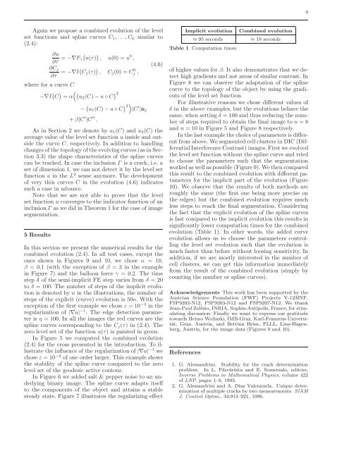
Implicit <strong>evolution</strong><br />
≈ 95 seconds<br />
Table 1 Computation times.<br />
<strong>Combined</strong> <strong>evolution</strong><br />
≈ 18 seconds<br />
<strong>of</strong> higher values <strong>for</strong> β. It also demonstrates that we detect<br />
high gradients <strong>and</strong> not areas <strong>of</strong> similar contrast. In<br />
Figure 8 we can observe the adaptation <strong>of</strong> the <strong>spline</strong><br />
curve to the topology <strong>of</strong> the object by using the gradients<br />
<strong>of</strong> the <strong>level</strong> set function.<br />
For illustrative reasons we chose different values <strong>of</strong><br />
δ in the above examples, but the <strong>evolution</strong>s behave the<br />
same, when setting δ = 100 <strong>and</strong> thus reducing the number<br />
<strong>of</strong> steps required to obtain the final image to n = 8<br />
<strong>and</strong> n = 10 in Figure 5 <strong>and</strong> Figure 8 respectively.<br />
In the last example the choice <strong>of</strong> parameters is different<br />
from above. We segmented cell clusters in DIC (Differential<br />
Interference Contrast) images. First we evolved<br />
the <strong>level</strong> set function without the <strong>spline</strong> curve <strong>and</strong> tried<br />
to choose the parameters such that the segmentation<br />
worked as well as possible (Figure 9). We then compared<br />
this result to the combined <strong>evolution</strong> with different parameters<br />
<strong>for</strong> the implicit part <strong>of</strong> the <strong>evolution</strong> (Figure<br />
10). We observe that the results <strong>of</strong> both methods are<br />
roughly the same (the first one being more precise on<br />
the edges) but the combined <strong>evolution</strong> requires much<br />
less steps to reach the final segmentation. Considering<br />
the fact that the explicit <strong>evolution</strong> <strong>of</strong> the <strong>spline</strong> <strong>curves</strong><br />
is fast compared to the implicit <strong>evolution</strong> this results in<br />
significantly lower computation times <strong>for</strong> the combined<br />
<strong>evolution</strong> (Table 1). In other words, the added curve<br />
<strong>evolution</strong> allows us to choose the parameters controlling<br />
the <strong>level</strong> set <strong>evolution</strong> such that the <strong>evolution</strong> is<br />
much faster than be<strong>for</strong>e without loosing sensitivity. In<br />
addition, if we are mostly interested in the number <strong>of</strong><br />
cell clusters, we can get this in<strong>for</strong>mation immediately<br />
from the result <strong>of</strong> the combined <strong>evolution</strong> (simply by<br />
counting the number or <strong>spline</strong> <strong>curves</strong>).<br />
Acknowledgements This work has been supported by the<br />
Austrian Science Foundation (FWF) Projects Y-123INF,<br />
FSP9202-N12, FSP9203-N12 <strong>and</strong> FSP9207-N12. We thank<br />
Jean-Paul Zolésio, INRIA, Sophia-Antipolis, France, <strong>for</strong> stimulating<br />
discussion. Finally we want to express our gratitude<br />
towards Heimo Wolinski, IMB-Graz, Karl-Franzens-Universität,<br />
Graz, Austria, <strong>and</strong> Bettina Heise, FLLL, Linz-Hagenberg,<br />
Austria, <strong>for</strong> the image data (Figures 9 <strong>and</strong> 10).<br />
References<br />
1. G. Aless<strong>and</strong>rini. Stability <strong>for</strong> the crack determination<br />
problem. In L. Päivärinta <strong>and</strong> E. Somersalo, editors,<br />
Inverse Problems in Mathematical Physics, volume 422<br />
<strong>of</strong> LNP, pages 1–8, 1993.<br />
2. G. Aless<strong>and</strong>rini <strong>and</strong> A. Diaz Valenzuela. Unique determination<br />
<strong>of</strong> multiple cracks by two measurements. SIAM<br />
J. Control Optim., 34:913–921, 1996.