Line Element Geometry for 3D Shape Understanding and ...
Line Element Geometry for 3D Shape Understanding and ...
Line Element Geometry for 3D Shape Understanding and ...

You also want an ePaper? Increase the reach of your titles
YUMPU automatically turns print PDFs into web optimized ePapers that Google loves.
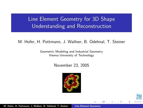
<strong>Line</strong> <strong>Element</strong> <strong>Geometry</strong> <strong>for</strong> <strong>3D</strong> <strong>Shape</strong><strong>Underst<strong>and</strong>ing</strong> <strong>and</strong> ReconstructionM. Hofer, H. Pottmann, J. Wallner, B. Odehnal, T. SteinerGeometric Modeling <strong>and</strong> Industrial <strong>Geometry</strong>Vienna University of TechnologyNovember 23, 2005M. Hofer, H. Pottmann, J. Wallner, B. Odehnal, T. Steiner <strong>Line</strong> <strong>Element</strong> <strong>Geometry</strong>
Task we want to solve . . .◮ Given: data set of a <strong>3D</strong> shape◮ Goal: underst<strong>and</strong> <strong>and</strong> reconstruct the special geometry◮ Tools: line elements <strong>and</strong> their relation to equi<strong>for</strong>m kinematicsM. Hofer, B. Odehnal, H. Pottmann, T. Steiner, J. Wallner: <strong>3D</strong>shape underst<strong>and</strong>ing <strong>and</strong> reconstruction based on line elementgeometry. Proc. ICCV’05, Vol. 2:1532–1538, 2005.M. Hofer, H. Pottmann, J. Wallner, B. Odehnal, T. Steiner <strong>Line</strong> <strong>Element</strong> <strong>Geometry</strong>
Task we want to solve . . .◮ Given: data set of a <strong>3D</strong> shape◮ Goal: underst<strong>and</strong> <strong>and</strong> reconstruct the special geometry◮ Tools: line elements <strong>and</strong> their relation to equi<strong>for</strong>m kinematicsM. Hofer, B. Odehnal, H. Pottmann, T. Steiner, J. Wallner: <strong>3D</strong>shape underst<strong>and</strong>ing <strong>and</strong> reconstruction based on line elementgeometry. Proc. ICCV’05, Vol. 2:1532–1538, 2005.M. Hofer, H. Pottmann, J. Wallner, B. Odehnal, T. Steiner <strong>Line</strong> <strong>Element</strong> <strong>Geometry</strong>
Task we want to solve . . .◮ Given: data set of a <strong>3D</strong> shape◮ Goal: underst<strong>and</strong> <strong>and</strong> reconstruct the special geometry◮ Tools: line elements <strong>and</strong> their relation to equi<strong>for</strong>m kinematicsM. Hofer, B. Odehnal, H. Pottmann, T. Steiner, J. Wallner: <strong>3D</strong>shape underst<strong>and</strong>ing <strong>and</strong> reconstruction based on line elementgeometry. Proc. ICCV’05, Vol. 2:1532–1538, 2005.M. Hofer, H. Pottmann, J. Wallner, B. Odehnal, T. Steiner <strong>Line</strong> <strong>Element</strong> <strong>Geometry</strong>
Task we want to solve . . .◮ Given: data set of a <strong>3D</strong> shape◮ Goal: underst<strong>and</strong> <strong>and</strong> reconstruct the special geometry◮ Tools: line elements <strong>and</strong> their relation to equi<strong>for</strong>m kinematicsM. Hofer, B. Odehnal, H. Pottmann, T. Steiner, J. Wallner: <strong>3D</strong>shape underst<strong>and</strong>ing <strong>and</strong> reconstruction based on line elementgeometry. Proc. ICCV’05, Vol. 2:1532–1538, 2005.M. Hofer, H. Pottmann, J. Wallner, B. Odehnal, T. Steiner <strong>Line</strong> <strong>Element</strong> <strong>Geometry</strong>
Equi<strong>for</strong>m kinematics & velocity vector fields◮ An equi<strong>for</strong>m trans<strong>for</strong>mationx ↦→ y = αAx + a, α > 0, A ∈ SO 3 , a ∈ R 3 .is a rigid body motion together with a scaling.◮ For a smooth equi<strong>for</strong>m motion, α, a, A depend smoothly on atime parameter t. Velocity vectors of points are given byẏ(t) = ( ˙αA + αȦ)x + ȧ = · · · = c × y + c + γy,with vectors c, c <strong>and</strong> a real number γ.◮ Use 7-tuple (c, c, γ) to encode velocity vector fields whichoccur with smooth equi<strong>for</strong>m motions.M. Hofer, H. Pottmann, J. Wallner, B. Odehnal, T. Steiner <strong>Line</strong> <strong>Element</strong> <strong>Geometry</strong>
Equi<strong>for</strong>m kinematics & velocity vector fields◮ An equi<strong>for</strong>m trans<strong>for</strong>mationx ↦→ y = αAx + a, α > 0, A ∈ SO 3 , a ∈ R 3 .is a rigid body motion together with a scaling.◮ For a smooth equi<strong>for</strong>m motion, α, a, A depend smoothly on atime parameter t. Velocity vectors of points are given byẏ(t) = ( ˙αA + αȦ)x + ȧ = · · · = c × y + c + γy,with vectors c, c <strong>and</strong> a real number γ.◮ Use 7-tuple (c, c, γ) to encode velocity vector fields whichoccur with smooth equi<strong>for</strong>m motions.M. Hofer, H. Pottmann, J. Wallner, B. Odehnal, T. Steiner <strong>Line</strong> <strong>Element</strong> <strong>Geometry</strong>
Equi<strong>for</strong>m kinematics & velocity vector fields◮ An equi<strong>for</strong>m trans<strong>for</strong>mationx ↦→ y = αAx + a, α > 0, A ∈ SO 3 , a ∈ R 3 .is a rigid body motion together with a scaling.◮ For a smooth equi<strong>for</strong>m motion, α, a, A depend smoothly on atime parameter t. Velocity vectors of points are given byẏ(t) = ( ˙αA + αȦ)x + ȧ = · · · = c × y + c + γy,with vectors c, c <strong>and</strong> a real number γ.◮ Use 7-tuple (c, c, γ) to encode velocity vector fields whichoccur with smooth equi<strong>for</strong>m motions.M. Hofer, H. Pottmann, J. Wallner, B. Odehnal, T. Steiner <strong>Line</strong> <strong>Element</strong> <strong>Geometry</strong>
Uni<strong>for</strong>m motions <strong>and</strong> Euclidean invariant surfaces◮ Uni<strong>for</strong>m motions have a constant velocity vector field.◮ The Euclidean ones (ẏ = c × y + c) are translations,rotations, <strong>and</strong> helical motions.◮ The corresponding invariant surfaces are cylindrical,rotational, <strong>and</strong> helical surfaces.M. Hofer, H. Pottmann, J. Wallner, B. Odehnal, T. Steiner <strong>Line</strong> <strong>Element</strong> <strong>Geometry</strong>
Uni<strong>for</strong>m motions <strong>and</strong> equi<strong>for</strong>m invariant surfaces◮ Uni<strong>for</strong>m motions have a constant velocity vector field.◮ The truly equi<strong>for</strong>m ones (ẏ = c × y + c + γy) are exponentialscaling <strong>and</strong> spiral motion.◮ The corresponding invariant surfaces are conical <strong>and</strong> spiraloidsurfaces.M. Hofer, H. Pottmann, J. Wallner, B. Odehnal, T. Steiner <strong>Line</strong> <strong>Element</strong> <strong>Geometry</strong>
<strong>Line</strong> elementsnyn◮ A line element is a line with a point yon it, encoded via a 7-tuple(n, n, ν) ∈ R 7 ,oνn . . . unit direction vector,n = y × n . . . moment vector,ν = 〈y, n〉 . . . scalar.M. Hofer, H. Pottmann, J. Wallner, B. Odehnal, T. Steiner <strong>Line</strong> <strong>Element</strong> <strong>Geometry</strong>
<strong>Line</strong> elements <strong>and</strong> equi<strong>for</strong>m kinematicsnyẏ◮ Look <strong>for</strong> “path normal elements”orthogonal to velocity vectors of asmooth equi<strong>for</strong>m motion.◮ Fact. A line element (n, n, ν) is apath normal element of the velocityvector field ẏ = c × y + c + γy iff¯n = y × n, ν = 〈y, n〉〈n, c〉 + 〈n, c〉 + νγ = 0.M. Hofer, H. Pottmann, J. Wallner, B. Odehnal, T. Steiner <strong>Line</strong> <strong>Element</strong> <strong>Geometry</strong>
<strong>Line</strong> elements <strong>and</strong> equi<strong>for</strong>m kinematicsnyẏ◮ Look <strong>for</strong> “path normal elements”orthogonal to velocity vectors of asmooth equi<strong>for</strong>m motion.◮ Fact. A line element (n, n, ν) is apath normal element of the velocityvector field ẏ = c × y + c + γy iff¯n = y × n, ν = 〈y, n〉〈n, c〉 + 〈n, c〉 + νγ = 0.M. Hofer, H. Pottmann, J. Wallner, B. Odehnal, T. Steiner <strong>Line</strong> <strong>Element</strong> <strong>Geometry</strong>
<strong>Line</strong> elements <strong>and</strong> equi<strong>for</strong>m kinematicsnyẏ◮ Look <strong>for</strong> “path normal elements”orthogonal to velocity vectors of asmooth equi<strong>for</strong>m motion.◮ Fact. A line element (n, n, ν) is apath normal element of the velocityvector field ẏ = c × y + c + γy iff¯n = y × n, ν = 〈y, n〉〈n, c〉 + 〈n, c〉 + νγ = 0.M. Hofer, H. Pottmann, J. Wallner, B. Odehnal, T. Steiner <strong>Line</strong> <strong>Element</strong> <strong>Geometry</strong>
Recognizing invariant surfacesTheoremThe coordinates (n, n, ν) of the normalline elements of a surface fulfill a linearhomogeneous equation〈n, c〉 + 〈n, c〉 + νγ = 0⇐⇒ the surface is invariant w.r.t. theuni<strong>for</strong>m motion determined by thevelocity vector fieldẏ = c × y + c + γy.M. Hofer, H. Pottmann, J. Wallner, B. Odehnal, T. Steiner <strong>Line</strong> <strong>Element</strong> <strong>Geometry</strong>
Classification of invariant surfaces – the exact case1. Given surface sample points y i with unit surface normalvectors n i , compute corresponding normal line elements(n i , n i , ν i ) with n i = y i × n i , ν i = 〈y i , n i 〉.2. Find all linear homogeneous equationsfulfilled by normal elements.〈n i , c〉 + 〈n i , c〉 + ν i γ = 0.3. Each such (c, c, γ) means a uni<strong>for</strong>m motion which leaves thesurface invariant. Some surfaces are multiply invariant.M. Hofer, H. Pottmann, J. Wallner, B. Odehnal, T. Steiner <strong>Line</strong> <strong>Element</strong> <strong>Geometry</strong>
Classification of invariant surfaces – the exact case1. Given surface sample points y i with unit surface normalvectors n i , compute corresponding normal line elements(n i , n i , ν i ) with n i = y i × n i , ν i = 〈y i , n i 〉.2. Find all linear homogeneous equationsfulfilled by normal elements.〈n i , c〉 + 〈n i , c〉 + ν i γ = 0.3. Each such (c, c, γ) means a uni<strong>for</strong>m motion which leaves thesurface invariant. Some surfaces are multiply invariant.M. Hofer, H. Pottmann, J. Wallner, B. Odehnal, T. Steiner <strong>Line</strong> <strong>Element</strong> <strong>Geometry</strong>
Classification of invariant surfaces – the exact case1. Given surface sample points y i with unit surface normalvectors n i , compute corresponding normal line elements(n i , n i , ν i ) with n i = y i × n i , ν i = 〈y i , n i 〉.2. Find all linear homogeneous equationsfulfilled by normal elements.〈n i , c〉 + 〈n i , c〉 + ν i γ = 0.3. Each such (c, c, γ) means a uni<strong>for</strong>m motion which leaves thesurface invariant. Some surfaces are multiply invariant.M. Hofer, H. Pottmann, J. Wallner, B. Odehnal, T. Steiner <strong>Line</strong> <strong>Element</strong> <strong>Geometry</strong>
Invariant surfaces◮ Classification of invariant surfaces using ẏ = c × y + c + γy:c = 0 c = 0 c ≠ 0 c ≠ 0 c ≠ 0γ = 0 γ ≠ 0 γ = 0 γ = 0 γ ≠ 0〈c, c〉 = 0 〈c, c〉 ≠ 0cylindrical conical rotational helical spiral surf.◮ Multiply invariant surfaces fall into two or more of theseclasses simultaneously.M. Hofer, H. Pottmann, J. Wallner, B. Odehnal, T. Steiner <strong>Line</strong> <strong>Element</strong> <strong>Geometry</strong>
Multiply invariant surfaces◮ Surfaces invariant with respect to ≥ 2 uni<strong>for</strong>m motions:cone (2) rot. cyl. (2) log. cyl. (2) sphere (3) plane (4)◮ logarithmic cylinder = cylinder with logarithmic spiral as basecurve (does not occur in applications)rot.M. Hofer, H. Pottmann, J. Wallner, B. Odehnal, T. Steiner <strong>Line</strong> <strong>Element</strong> <strong>Geometry</strong>
Surface recognition using PCA – the real world case◮ Normal line elements of a surface shaped noisy point set <strong>for</strong>ma point cloud (n i , n i , ν i ) in R 7 .◮ Fit a hyperplane 〈c, n〉 + 〈c, n〉 + νγ = 0 by minimizingF (c, c, γ) = ∑ Ni=1 (〈c, n i〉 + 〈c, n i 〉 + ν i γ) 2 .under the side condition c 2 + c 2 + γ 2 = 1.M. Hofer, H. Pottmann, J. Wallner, B. Odehnal, T. Steiner <strong>Line</strong> <strong>Element</strong> <strong>Geometry</strong>
Surface recognition using PCA – the real world case◮ Normal line elements of a surface shaped noisy point set <strong>for</strong>ma point cloud (n i , n i , ν i ) in R 7 .◮ Fit a hyperplane 〈c, n〉 + 〈c, n〉 + νγ = 0 by minimizingF (c, c, γ) = ∑ Ni=1 (〈c, n i〉 + 〈c, n i 〉 + ν i γ) 2 .under the side condition c 2 + c 2 + γ 2 = 1.M. Hofer, H. Pottmann, J. Wallner, B. Odehnal, T. Steiner <strong>Line</strong> <strong>Element</strong> <strong>Geometry</strong>
Surface recognition using PCA – the real world case◮ Quality of fit corresponds to magnitude of eigenvalues ofcovariance matrix∑ Ni=1 (n i, n i , ν i )(n i , n i , ν i ) T ∈ R 7×7 .Solution is given by a corresponding eigenvector (c, c, γ).◮ One small eigenvalue → invariant surface.◮ Two small eigenvalues → twofold invariant surface.M. Hofer, H. Pottmann, J. Wallner, B. Odehnal, T. Steiner <strong>Line</strong> <strong>Element</strong> <strong>Geometry</strong>
Surface recognition using PCA – the real world case◮ Quality of fit corresponds to magnitude of eigenvalues ofcovariance matrix∑ Ni=1 (n i, n i , ν i )(n i , n i , ν i ) T ∈ R 7×7 .Solution is given by a corresponding eigenvector (c, c, γ).◮ One small eigenvalue → invariant surface.◮ Two small eigenvalues → twofold invariant surface.M. Hofer, H. Pottmann, J. Wallner, B. Odehnal, T. Steiner <strong>Line</strong> <strong>Element</strong> <strong>Geometry</strong>
Axis <strong>and</strong> center of a spiral surfaceFrom (c, c, γ) compute axis (a, a) <strong>and</strong> center z ofequi<strong>for</strong>m motion:a = c,a =1γ 2 + c 2 (c2 c − 〈c, c〉c + γc × c),z =1γ(c 2 + γ 2 ) (γc × c − γ2 c − 〈c, c〉c).M. Hofer, H. Pottmann, J. Wallner, B. Odehnal, T. Steiner <strong>Line</strong> <strong>Element</strong> <strong>Geometry</strong>
Does nature produce exact spiral surfaces?◮ Given laser scanner data of a sea shell (Turbo Marmoratus)◮ Axes <strong>and</strong> centers cluster in piecewise reconstruction:M. Hofer, H. Pottmann, J. Wallner, B. Odehnal, T. Steiner <strong>Line</strong> <strong>Element</strong> <strong>Geometry</strong>
Reconstruction: Generator curves<strong>Shape</strong> of invariant surfaces is determined by a generator curve.M. Hofer, H. Pottmann, J. Wallner, B. Odehnal, T. Steiner <strong>Line</strong> <strong>Element</strong> <strong>Geometry</strong>
Example: Saxidomus NutalliM. Hofer, H. Pottmann, J. Wallner, B. Odehnal, T. Steiner <strong>Line</strong> <strong>Element</strong> <strong>Geometry</strong>
Example: Helix PomataM. Hofer, H. Pottmann, J. Wallner, B. Odehnal, T. Steiner <strong>Line</strong> <strong>Element</strong> <strong>Geometry</strong>
Segmentation procedureRANSAC is used <strong>for</strong> detecting1. Planar <strong>and</strong> spherical parts.2. Twofold invariant parts.3. Parts with simple invariance.M. Hofer, H. Pottmann, J. Wallner, B. Odehnal, T. Steiner <strong>Line</strong> <strong>Element</strong> <strong>Geometry</strong>
Segmentation & Morphology◮ If normal vectors fit into a rotation → surface part withrotational symmetry is detected.◮ Curve-like surface parts where the surface normals fit thesame rotation are removed, by morphological opening.M. Hofer, H. Pottmann, J. Wallner, B. Odehnal, T. Steiner <strong>Line</strong> <strong>Element</strong> <strong>Geometry</strong>
Conclusion◮ <strong>Line</strong> element geometry <strong>and</strong> equi<strong>for</strong>m kinematics together withnumerical/statistic techniques (PCA <strong>and</strong> RANSAC) arebeneficial <strong>for</strong> recognizing, reconstructing, <strong>and</strong> segmentingspecial <strong>3D</strong> shapes.◮ Applications are in engineering, archeology, <strong>and</strong> life sciences.M. Hofer, H. Pottmann, J. Wallner, B. Odehnal, T. Steiner <strong>Line</strong> <strong>Element</strong> <strong>Geometry</strong>
References◮ M. Hofer, B. Odehnal, H. Pottmann, T. Steiner, J. Wallner:<strong>3D</strong> shape underst<strong>and</strong>ing <strong>and</strong> reconstruction based on lineelement geometry. Proc. ICCV’05, Vol. 2:1532–1538, 2005.◮ H. Pottmann, M. Hofer, B. Odehnal, J. Wallner: <strong>Line</strong>geometry <strong>for</strong> <strong>3D</strong> shape underst<strong>and</strong>ing <strong>and</strong> reconstruction. InT. Pajdla <strong>and</strong> J. Matas, editors, Computer Vision - ECCV’04,Part I, LNCS 3021, pages 297-309, Springer, 2004.◮ B. Odehnal, H. Pottmann, J. Wallner: Equi<strong>for</strong>m kinematics<strong>and</strong> the geometry of line elements. Submitted to:Contributions to Algebra <strong>and</strong> <strong>Geometry</strong>.M. Hofer, H. Pottmann, J. Wallner, B. Odehnal, T. Steiner <strong>Line</strong> <strong>Element</strong> <strong>Geometry</strong>