Projectiles in a Uniform Gravitational Field

Projectiles in a Uniform Gravitational Field
1. Equations and Coordinate System
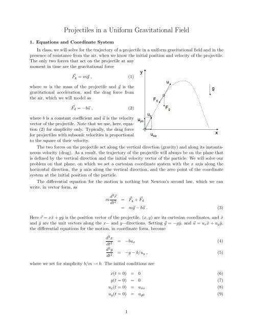
In class, we will solve for the trajectory of a projectile in a uniform gravitational field and in the
presence of resistance from the air, when we know the initial position and velocity of the projectile.
The only two forces that act on the projectile at any
moment in time are the gravitational force
⃗F g = m⃗g , (1)
where m is the mass of the projectile and ⃗g is the
gravitational acceleration, and the drag force from
the air, which we will model as
⃗F d = −b⃗u , (2)
where b is a constant coefficient and ⃗u is the velocity
vector of the projectile. Note that we use, here, equation
(2) for simplicity only. Typically, the drag force
for projectiles with subsonic velocities is proportional
to the square of their velocity.
The two forces on the projectile act along the vertical direction (gravity) and along its instantaneous
velocity (drag). As a result, the trajectory of the projectile will always be on the plane that
is defined by the vertical direction and the initial velocity vector of the particle. We will solve our
problem on that plane, on which we set a cartesian coordinate system with the x axis along the
horizontal direction, the y axis along the vertical direction, and the zero point of the coordinate
system at the initial position of the particle.
The differential equation for the motion is nothing but Newton’s second law, which we can
write, in vector form, as
m d2 ⃗r
dt 2 = ⃗ F g + ⃗ F d
= m⃗g − b⃗u . (3)
Here ⃗r = xˆx + yŷ is the position vector of the projectile, (x, y) are its cartesian coordinates, and ˆx
and ŷ are the unit vectors along the x− and y−directions. Setting ⃗g = −gŷ, and ⃗u = u xˆx + u y ŷ,
the differential equations for the motion, in coordinate form, become
where we set for simplicity b/m → b. The initial conditions are
d 2 x
dt 2 = −bu x (4)
d 2 y
dt 2 = −g − b/u y , (5)
x(t = 0) = 0 (6)
y(t = 0) = 0 (7)
u x (t = 0) = u xo (8)
u y (t = 0) = u y0 (9)
1

2. Converting Equations to Dimensionless Form
In order to convert the equations to a dimensionless form, we will start by considering the
units of the independent and dependent variables. In the problem we are studying, there is one
independent variable t of time units, i.e., [t]=[T], and two dependent variables, x, and y, of length
unit [L], i.e., [x]=[L] and [y]=[L]. This means that we will need to come up with a unit of time, t 0 ,
and a unit of length, l 0 .
We will construct the natural units of the problem by looking at (a) the initial conditions, and
(b) the parameters in the equation. In our problem, there are two initial conditions in coordinates
of length units, i.e., [x 0 ]=[L], and [y 0 ]=[L], and two in velocities, of units [u x0 ]=[L]/[T] and
[u y0 ]=[L]/[T]. Finaly, there are two parameters, b, and g, of units [b]=1/[T], and [g]=[L]/[T] 2 .
The initial conditions in coordinates are (x 0 , y 0 ) = (0, 0) and, therefore, are not useful in
defining the natural units of the problem. Using the other conditions and parameters, there are
two possibilites of defining a natural unit of time, since
[b −1 ]
= [T ] (10)
g
= [T ] . (11)
[ uy0
(Note that, in this last equation, we could have used the initial velocity in the x-direction, as well.)
We will use our understanding of the physics of the problem to choose among the two possibilities.
The time defined by b −1 is the characteristic timescale for the air resistance to slow down the
projectile. On the other hand, the time defined by u y0 /g is the characteristic timescale for gravity
to accelerate or deccelerate the projectile. For most applications, gravity is the dominant force,
and the latter timescale is the fastest. We, therefore, choose
t 0 = u y0
g
(12)
as our unit of time. We can the choose
l 0 = u2 y0
g . (13)
as our unit of length. Finally, having chosen a unit of length and a unit of time, it is also natural
to choose
u 0 = u y (14)
as the unit of velocity.
We now set
and convert the system of equations to
t ′ = t/t 0 (15)
x ′ = x/l 0 (16)
y ′ = y/l 0 (17)
u ′ x = u x /u 0 (18)
u ′ y = u y /u 0 (19)
d 2 x ′
dt ′2 = −Au ′ x (20)
d 2 y ′
dt 2 = −1 − Au ′ y , (21)
2

where we have defined a new dimensionless parameter
The dimensionless initial conditions are
A = bv y
g . (22)
x ′ 0 = y′ 0 = 0 (23)
u ′ x0 = u x0
u y0
≡ tan θ (24)
u ′ y0 = 1 . (25)
Clearly, the differential equation depends only on the parameter A and the boundary conditions
only on the initial angle with respect to the horizontal axis, θ.
3. Seting-up the Numerical Method
In order to solve the above system of 2nd order ODEs with the Runge-Kutta method, we need
to convert them to a system of 1st order ODEs. To this end we can use the definition of the
velocities along the x− and y− axes and rewrite the system as
with the same initial conditions
dx ′
dt ′ = v x ′ (26)
dv x
′
dt ′ = −Av x ′ (27)
dy ′
dt ′ = v y ′ (28)
dv y
′
dt ′ = −1 − Av y ′ (29)
x ′ 0 = y′ 0 = 0 (30)
u ′ x0 = u x0
u y0
≡ tan θ (31)
u ′ y0 = 1 . (32)
3