1 Exercise: Solving ODEs – Lorenz equations - USC Geodynamics

1 EXERCISE:SOLVINGODES –LORENZEQUATIONS
1 Exercise: SolvingODEs–Lorenzequations
Reading
• Spiegelman(2004),chap. 4
• Pressetal.(1993), chap. 17(16 in 2 nd ed.)
• Spencerand Ware(2008), sec. 16
We previously discussed the 4 th order Runge Kutta method as a simple method to
solve initial value problems where the task is to forward integrate a vector y(t) from an
initial condition y 0 (t = t 0 ) to some time t f while the time derivatives of y are given by
dy
(t) = f(t,y,C) (1)
dt
we madethe dependenceof f on constant parameters explicitin the C.
Numerically, this is done by successively computing y n+1 for time t +h from the last
known solution for y n attime t with time step h
y n+1 ≈ y n +hy ′ (h,t,y,C) (2)
where y ′ denotes the approximate time-derivatives for y.
Inarealapplication,wewoulduseadaptivestep-sizecontrolbymeansoferrorchecking
dependingon the accuracy of our approximate method, or employ an entirely different
approach (Press et al., 1993). Spencer and Ware (2008) discuss some of the algorithms
that are implemented in Matlab, and the problem set file rikitake.m 1 is an example
for how to use the Matlab function ode45. However, the Runge-Kutta is good example
method and easyenough to implement.
1.1 TheLorenz equations solved withsimple Runge Kutta
As an interesting example of a three-dimensional (y = {y 1 ,y 2 ,y 3 }) ODE system are the
Lorenz (1963) equations. These equations are a simplified description of thermal convection
in the atmosphere and an exampleof alow order, spectral numerical solution.
1 AllMatlabfilesfortheproblemsetsareathttp://geodynamics.usc.edu/~becker/teaching-557.html;
solutions areavailablefor instructors uponrequest.
USCGEOL557: ModelingEarth Systems 1

1 EXERCISE:SOLVINGODES –LORENZEQUATIONS
1.2 Digression for background – not essential to solving this problem
set
For anincompressible fluid, conservation of mass, energy,and momentum for the convection problemcan
bewritten as
∇ ·v = 0 (3)
∂T
∂t +v·∇T = κ∇2 T (4)
∂v
∂t + (v · ∇)v = ν∇2 v − 1 ∇P + ρ g.
ρ 0 ρ 0
(5)
Here, ν = η/ρ 0 is dynamic viscosity, v velocity, T temperature, κ thermal diffusivity, g gravitational acceleration,
ρ density, and P pressure. In the Boussinesq approximation, ρ(T) = ρ 0 (1 − α(T −T 0 )), where α is
thermal expansivityand ρ 0 and T 0 referencedensity andtemperature,respectively.
If we assume two-dimensionality (2-D) in x and z direction, and a bottom-heated box of fluid, the
box height d provides a typical length scale. If g only acts in z direction and all quantities are nondimensionalized
by d, the diffusion time, d 2 /κ, and the temperature contrast between top and bottom
∆T,we canwrite
1
Pr
∂T ′
∂t ′ +v ′ · ∇T ′ = ∇ 2 T ′ (6)
( )
∂ω
∂t ′ +v ′ · ∇ω = ∇ 2 ω −Ra ∂T′
∂x ′ , (7)
where the primed quantities are non-dimensionalized (more on this later). Eq. (7) is eq. (5) rewritten in
terms of vorticity ω,suchthat ∇ 2 ψ = −ω where ψ is the stream-function,whichrelatestovelocity as
v = ∇ × ψk = {∂ψ/∂z, −∂ψ/∂x} (8)
andenforcesincompressibility(massconservation). Theimportantpartherearethetwonewnon-dimensional
quantities that arise, the Prandtl and the Rayleigh numbers, which were discussed previously (eqs. ?? and
??).
Lorenz (1963)used a very low orderspectral expansion to solve the convection equations. He assumed
that
ψ ≈ W(t)sin (πax)sin (πz) (9)
T ≈ (1 −z) +T 1 (t)cos(πax)sin (πz) +T 2 (t)sin(2πz) (10)
for convective cells with wavelength2/a. This is anexampleof a spectralmethod wherespatial variations
in properties such as T are dealt with in the frequency domain, here with one harmonic. Such an analysis
is alsocommon when examining barelysuper-criticalconvectiveinstabilities.
1.3 Problems
The resulting equations for the time dependent parameters of the approximate Lorenz
convection equationsare
dW
dt
dT 1
dt
dT 2
dt
= Pr(T 1 −W) (11)
= −WT 2 +rW −T 1
= WT 1 −bT 2
USCGEOL557: ModelingEarth Systems 2

1 EXERCISE:SOLVINGODES –LORENZEQUATIONS
where b = 4/(1 +a 2 ), r = Ra/Ra c with the critical Rayleigh number Ra c .
1. IdentifyW, T 1 , and T 2 as y 1 ,y 2 ,y 3 and write up a Matlab code for a4 th orderRunge
Kutta scheme to solve for the time-evolution of y usingeq. (11)forderivatives.
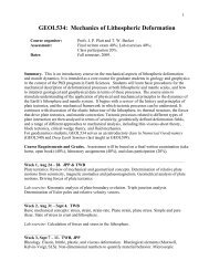
Hint: You can code this anywayyou want, but considerthe following (Figure 2):
• You will wantto separate a “driver” that dealswith initial conditions, controlling
the total time steps, plotting, etc., and an actual routine that computes the
Runge Kutta step following the formula we discussed in class. Those should
be separate m-files, or atleastseparate functions.
• YouwillwanttomaketheRungeKuttastepperindependentoftheactualfunctionthatisneededtocomputedy/dtsothatyoucanreuseitforotherproblems
later. This can be done in Matlab by defining a function myfunc that computes
the derivatives, and then passing the function name myfunc as an argument to
the Runge Kutta time stepper. Within the time stepper, the function then then
hasto be referred toas
@func. Alternatively, the function that computes the derivatives can be made
intoitsown “.m”file,inthe samedirectory astheothersubroutines, makingit
available to allsubroutines in that folder.
• Ifyouneedsomeinspirationonhowtodothis,downloadthem-filefragments
we provide for thissections problem set,dydt.m, lorenz.m, andrkstep.m.
2. Use initial condition y 0 = {0,0.5,0.5}, parameters b = 8/3, Pr = 10 and solve
for time evolution for all three variables from t = 0 to t = 50, using a time step
h = 0.005. Use r = 2 and plot T 1 and T 2 against time. Comment on the temporal
character ofthe solution, whatdoesitcorrespond to physically?
3. Change r to 10, and then 24. Plot T 1 and T 2 against time, and also plot the “phase
space trajectory” of the system by plotting y in W, T 1 , and T 2 space using Matlab
plot3. Commenton how these solutions differ.
4. Increase r to 25 and plot both time behavior of T and the phase space trajectory.
What happened? Compare the r = 25 solution with the r = 24 solution from the
lastquestion. Doyouthinkr = 24willremainsteadyforalltimes? Why? Whynot?
5. Use r = 30 and show on one plot how T 1 evolves with time for two different
initial conditions, the y 0 from before, {0,0.5,0.5}, and a second initial condition
{0,0.5,0.50001}. Comment.
6. Compareyoursolution with h = 0.005for T 1 andaninitialcondition ofyourchoice
inther = 30regimewiththeMatlab-internalODEsolveryoudeemmostappropriate.
Plot the absolute difference ofthe solutions against time. Comment.
USCGEOL557: ModelingEarth Systems 3

1 EXERCISE:SOLVINGODES –LORENZEQUATIONS
T 2
50
45
40
35
30
25
20
15
10
5
0
30
20
10
T 1
0
−10
−20
−15
−10
−5
0
W
5
10
15
20
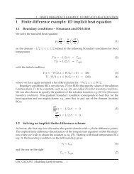
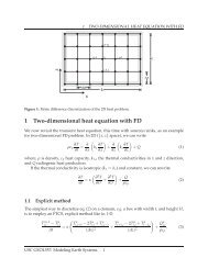
Figure1: SolutiontooneoftheproblemsetquestionsvisualizingthebehavioroftheLorenz
equations(theLorenzattractor).
ForhelpwithmakingsimpleplotswithMatlab,seeSpencerandWare(2008),forexample.
1.4 Additional examples
1. IfyouarecuriousaboutadditionalEarthScienceapplicationsofODEs,theliterature
ofgeochemical modelingis full ofit because itis often easiest, or most appropriate,
to consider fluxes between reservoirs of different chemical species with averages
properties, so-called “box models” (e.g.Albarede,1995).
2. Aclassicexamplefrommagneto-hydrodynamicsisthe3-DRikitakedynamomodel
that consists of two conducting, coupled rotating disks in a background magnetic
field. TheRikitakedynamoshowsbehaviorsimilartotheLorenzsystemandserves
asan analogfor magneticfield reversal. The equationsare
dx
dt
dy
dt
dz
dt
= −mx +yz (12)
= −my + (z −a)x
= 1 −xy
with typical parametersfor a of4or10, m = 2,atinitial conditions x,y,z = −5,2,2.
USCGEOL557: ModelingEarth Systems 4

1 EXERCISE:SOLVINGODES –LORENZEQUATIONS
function lorenz % this is only a function to allow function declarations
%
% Lorent’z equation solver
% the ... parts will have to be filled in by you
%
% values to solve for
%
% y(1) : W
% y(2) : T1
% y(3) : T2
% parameters for the equations
parameters.r = ...; % Rayleigh number
parameters.Pr = ..; % Prandtl number
% initial values
y= [...];
time =0;tstop=50;
h = 0.005;% timestep
save_each = 1;
nstep=0;save_step=0;
while(time < tstop) % loop while time is smaller than tstop
if(mod(nstep,save_each)==0) % only save every save_each step
save_step=save_step+1;
ysave(save_step,:)=y;
...
end
% advance the y(1:3) solution by one 4th order Runge Kutta step
y = y + rkstep(....);
nstep=nstep+1;
time=time+h;
end
figure(1);clf % time series
plot(tsave,ysave(:,2))
xlabel(’time’);ylabel(’temperature’);
legend(’T_1’,’T_2’)
function dy = rkstep(.... )
%
%
% perform one 4th order Runge Kutta timestep and return
% the increment on y(t_n) by evaluating func(time,y,parameters)
%
% ... parts need to be filled in
%
%
% input values:
% h: time step
% t: time
% y: vector with variables at time = t which are to be advanced
% func: function which computes dy/dt
% parameters: structure with any parameters the func function might need
% save computations
h2=h/2;
k1 = h .* dydt(...);
k2 = h .* dydt(...);
....
% return the y_{n+1} timestep
dy = ....
function dydt = lorenz_dy(...)
%
% functions for Runge Kutta
%
%
% dW/dt = Pr (T1-w)
%
dydt(1) = ...
%
% dT1/dt = -W T2 + rW - T1
%
dydt(2) = ...
%
% dT2/dt = W T1 - b T2
%
dydt(3) = ... x
Figure 2: Suggested program structure for the Lorenz equation ODE solver exercise. Available
online aslorenz.m,rkstep.m,anddydt.m.
USCGEOL557: ModelingEarth Systems 5

1 EXERCISE:SOLVINGODES –LORENZEQUATIONS
The file rikitake.m provides an example implementation of these equations using
a MatlabODE solver.
3. Examples from our own research where we have used simple ODE solutions, include
some work on parameterized convection (Loyd et al., 2007), a method that
goes back at least to Schubert et al. (1980), see Christensen (1985). In this case, the
box is the mantle, and the total heat content of the mantle, as parameterized by the
mean temperature, is the property one solves for. I.e. we are averaging the PDEs
governing convection spatially, to solve for the time-evolution of average mantle
temperature.
The ideaisthat aconvective system with Rayleigh number
Ra = ραTgh3
κη
(13)
transports heatatNusselt number Nu following a scaling of
Nu = Q cT = aRaβ (14)
(withsomedebateabout β,see,e.g.Korenaga,2008,forareview). Theenergybalance
for the mantle is
dT
C p = H(t) −Q (15)
dt
where C p is the total heat capacity, H the time-dependent heat production through
radiogenic elements, and Q the heat loss through the surface. If viscosity is a function
oftemperature,
then the equationscouple such that
C p
dT
dt = H(t) −Q 0
( H
η = η 0 exp
RT)
(16)
( ) T 1+β ( )
η(T0 ) β
. (17)
T 0 η(T)
Weprovideanexample,thermal_all.m online. Youmightwanttoexperimentwith
the shooting method to explore feasible and unfeasable paths of Earth’s thermal
evolution from an initial to afinal temperature.
4. Anotherexample,fromthebrittleregime,arespringsliders. Insteadofdealingwith
fullfaultdynamics,onemayconsiderablockthathasafrictionlawapplyatitsbase
and pulled by a string. Depending on the assumptions on the friction law, such a
system exhibits stick-slip behavior akin to the earthquake cycle. For rate-and-state
(i.e. velocity and heal-time) dependent friction (e.g. Marone, 1998) with two “state”
variables, spring-slider modelsexhibit interesting, chaotic behavior (Becker,2000).
USCGEOL557: ModelingEarth Systems 6

1 EXERCISE:SOLVINGODES –LORENZEQUATIONS
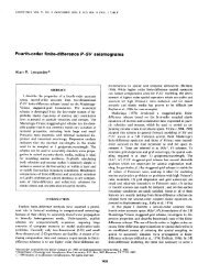
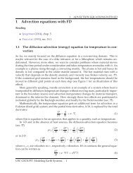
Figure 3: Poincare sections in y for the period doubling sequence to chaos for the springslider
system,eq. (18), as a function of normalized spring stiffness, κ ′ . Bottomfigure shows
zoom intothedashedrectangular regionhighlightedontop(modifiedfromBecker, 2000).
The equationsare
ẋ = dx
dt
ẏ = dy
dt
ż = dz
dt
= e x ((β 1 −1)x +y−z) +ẏ−ż (18)
= (1 −e x )κ
= −e x ρ(β 2 x +z)
with β 1 = 1, β 2 = 0.84,and ρ = 0.048(Guetal., 1984).
Thisbehaviorincludesthecharacteristicperiod-doublingroutetowardchaos(Feigenbaum,
1978) as a function of a material parameter (spring stiffness), at critical κ =
0.08028(Becker,2000). You mightwanttoreproduce thebifurcation plotofFigure 3.
USCGEOL557: ModelingEarth Systems 7

BIBLIOGRAPHY
Bibliography
Albarede,F. (1995), Introduction togeochemicalmodeling,Cambridge University Press.
Becker, T. W. (2000), Deterministic chaos in two state-variable friction sliders and the effectofelasticinteractions,inGeoComplexityandthephysicsofearthquakes,Geophys.Monograph,vol.
120, edited by J. B. Rundle,D. L. Turcotte, and W. Klein, pp. 5–26,American
Geophysical Union, Washington, DC.
Christensen, U. R. (1985), Thermal evolution models for the Earth, J. Geophys. Res., 90,
2995–3007.
Feigenbaum, M. J. (1978), Quantitative universality for a class of nonlinear transformations,
J. Stat. Phys.,19, 25.
Gu, J.-C., J. R. Rice, A. L. Ruina, and S. T. Tse (1984), Slip motion and stability of a single
degree of freedom elastic system with rate and state dependent friction, J. Mech. Phys.
Solids,32,167–196.
Korenaga, J. (2008), Urey ratio and the structure and evolution of Earth’s mantle, Rev.
Geophys.,46, doi:10.1029/2007RG000241.
Lorenz, E. N.(1963), Deterministic nonperiodic flow,J. Atmos. Sci.,20, 130.
Loyd, S. J., T. W. Becker, C. P. Conrad, C. Lithgow-Bertelloni, and F. A. Corsetti (2007),
Time-variability in Cenozoic reconstructions of mantle heat flow: plate tectonic cycles
andimplications forEarth’sthermal evolution, Proc.Nat. Acad.Sci.,104,14,266–14,271.
Marone,C.(1998),Laboratory-derivedfrictionlawsandtheirapplicationtoseismicfaulting,
Annu. Rev.Earth Planet. Sci.,26,643–696.
Press, W.H.,S.A.Teukolsky, W.T.Vetterling, andB.P.Flannery(1993),NumericalRecipes
inC: TheArtof ScientificComputing, 2ed., Cambridge UniversityPress, Cambridge.
Schubert,G.,D.Stevenson,andP.Cassen(1980),Wholeplanetcoolingandtheradiogenic
heatsource contents ofthe Earth and Moon, J. Geophys.Res., 85,2531–2538.
Spencer, R. L., and M. Ware (2008), Introduction to Matlab, Brigham Young University,
availableonline, accessed 07/2008.
Spiegelman, M. (2004), Myths and Methods in Modeling,
Columbia University Course Lecture Notes, available online at
http://www.ldeo.columbia.edu/~mspieg/mmm/course.pdf, accessed 06/2006.
USCGEOL557: ModelingEarth Systems 8