1 Wave propagation - USC Geodynamics

1 Wave propagation
1 WAVEPROPAGATION
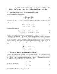
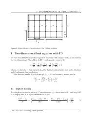
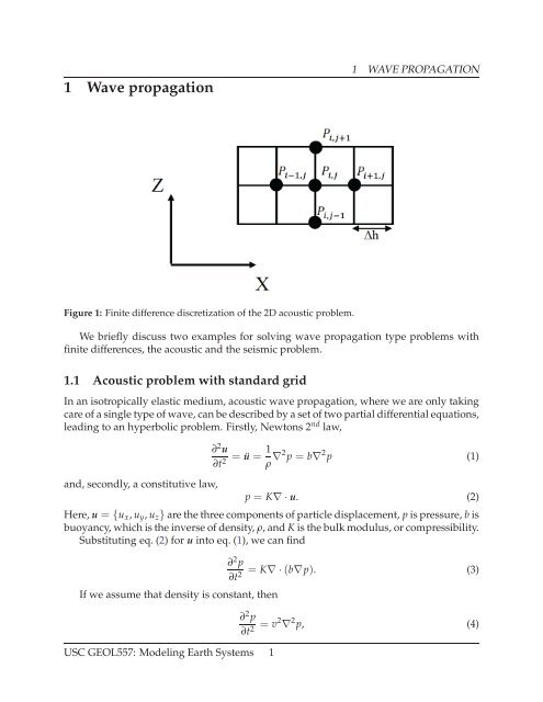
Figure1: Finitedifference discretization of the2D acousticproblem.
We briefly discuss two examples for solving wave propagation type problems with
finite differences, the acoustic and the seismicproblem.
1.1 Acoustic problemwithstandardgrid
In an isotropically elastic medium, acoustic wave propagation, where we are only taking
careofasingletypeofwave,canbedescribedbyasetoftwopartialdifferentialequations,
leadingtoan hyperbolic problem. Firstly, Newtons 2 nd law,
and,secondly, a constitutive law,
∂ 2 u
∂t 2 = ü = 1 ρ ∇2 p = b∇ 2 p (1)
p = K∇ ·u. (2)
Here,u = {u x ,u y ,u z }arethethreecomponentsofparticledisplacement, pispressure,bis
buoyancy,whichistheinverseofdensity, ρ,andKisthebulkmodulus,orcompressibility.
Substituting eq.(2)for u into eq.(1), we can find
Ifwe assume thatdensity isconstant, then
USCGEOL557: ModelingEarth Systems 1
∂ 2 p
= K∇ · (b∇p). (3)
∂t2 ∂ 2 p
∂t 2 = v2 ∇ 2 p, (4)

1 WAVEPROPAGATION
where
v = √ Kb =
√
K
ρ
denotesthe bulk sound velocity. Simplifying toa2Dcase, wehave
∂ 2 (
p
∂
∂t 2 = v2 (x,z)
2 )
p
∂x 2 + ∂2 p
∂z 2 . (6)
The equation for propogation of SH waves, the transverse components of S waves, in
seismology hasasimilar form aseq. (6):
∂ 2 (
u
∂
∂t 2 = v2 SH (x,z) 2 )
u
∂x 2 + ∂2 u
∂z 2 , (7)
where u isthe displacementandV SH isthe velocity of the SH component.
Likewise, a similar equation also applies for tsunami waves at long wavelengths, in
the “shallow water approximation”,
∂ 2 (
ξ
∂ 2 )
∂t 2 = ξ
v2 (x,z)
∂x 2 + ∂2 ξ
∂z 2 . (8)
Here, ξ is the height of the tsunami wave, v is the velocity defined by the water depth H
as
v = √ gH. (9)
To solve equations (6)-(8), with finite differences, we use the mesh shown in Fig. 1.
Here, we have p n i,j
= P(i∆h,j∆h,n∆t) and v i,j = v(i∆h,j∆h). Applying the 2 nd -order,
second derivative formula to the acoustic waveequation eq.(6),
p n−1
i,j
−2pi,j n + pn+1 i,j
∆t 2
= v 2 i,j
[ p
n
i−1,j
−2p n i,j + pn i+1,j
∆h 2
(5)
+ pn i,j−1 −2pn i,j + ]
pn i,j+1
∆h 2 . (10)
Afterrearranging, wehave
(
)
p n+1
i,j
= −p n−1
i,j
+ (2 −4a i,j )2pi,j n +a i,j pi−1,j n + pn i+1,j + pn i,j−1 + pn i,j+1 , (11)
where
a i,j = v 2 ∆h 2
i,j
∆t2. (12)
Then, the pressure ordisplacementattime step n +1can be derived explicitly from time
step n and n −1 asin eq.(11), though two solutions have tobe stored.
Note that we use 2 nd -order second derivatives in eq. (11). Two considerations are requiredforchoosingsuitabletimestep
∆tandspatialstep ∆h: griddispersionandstability.
USCGEOL557: ModelingEarth Systems 2

1 WAVEPROPAGATION
When waves propagate on a discrete grid, they produces an artificial variation of velocity
withfrequency, whichiscalledgriddispersion. Thehigherfrequencysignals,with
slower velocity, are delayed relative to the lower frequency arrivals. This dispersion increases
as ∆h becomes larger. In other words, a small ∆h is required to avoid grid dispersion.
To achieve an accurate solution, we need at least 12 points per wavelength for space
foraschemewith2 nd orderaccuracy. Fora4 th orderscheme,aminimumof6.5pointsper
wavelength arerequired. For afixedfrequency, thisminimumwavelength isdetermined
by the minimum velocity (v min ), so the accuracy of the system is governed by (v min ).
Following astability analysis, we can derivethe stability requirementhere as:
∆t ≤
1 √
2
∆h
v max
(13)
where v max isthe maximum velocity on the grid.
1.1.1 Exercise1
• Program the 2D acoustic wave propagation in standard grid scheme as in Fig. 1
(wave_acoustic_2D.m). Study the wavefield and seismograms with different choicesof
∆t and ∆h anddemonstrate how ∆t and ∆h affectthe stability andgrid dispersion
in the program.
• Introduceheterogeneitiesinthevelocities,suchasathinlayerwithhalfvelocity,and
describethedifferencefromtheisotropicmodel,especiallyhowthislayeraffectsthe
observed seismograms. Run the code with the velocity inside the thin layer being
zeroand explain the result.
1.2 Elasticwave problemwithstaggeredgrid
For 2Delasticwave case (P-SV system), we have the equationsas:
ρ ∂2 u x
∂t 2 = ∂τ xx
∂x + ∂τ xz
∂z , (14)
ρ ∂2 u z
∂t 2 = ∂τ xz
∂x + ∂τ zz
∂z , (15)
τ xx = (λ +2µ) ∂u x
∂x + λ∂u z
∂z , (16)
and
τ zz = (λ +2µ) ∂u z
∂z + λ∂u x
∂x , (17)
( ∂ux
τ xz = µ
∂z + ∂u )
z
. (18)
∂x
USCGEOL557: ModelingEarth Systems 3

1 WAVEPROPAGATION
Here, (u x ,u z ) are the particle displacements. For seismic waves, they are typically called
radial and vertical components, respectively, if they are recorded at surface. Further, τ is
thestresstensor,and λ(x,z)and µ(x,z)theelastic,Lamécoefficients(µisshearmodulus).
Typically, those equations are solved for particle velocities as u = ∂u x
∂t
and v = ∂u z
∂t . Then,
the system istransformed into the frst-order hyperbolic system:
(
∂u
∂t = b ∂τxx
∂x + ∂τ xz
∂z
(
∂v
∂t = b ∂τxz
∂x + ∂τ zz
∂z
)
, (19)
)
, (20)
∂τ xx
= (λ +2µ) ∂u
∂t
∂x + λ∂v ∂z , (21)
∂τ zz
= (λ +2µ) ∂v
∂t
∂x + λ∂u ∂z , (22)
(
∂τ xz ∂u
= µ
∂t ∂z + ∂v )
. (23)
∂x
Atypicalseismicwavepropagationproblemneedstodealwithmediumwithvariable
Poisson’s ratio, ν, which can be definedas
ν =
λ
2(λ + µ) . (24)
For the special case of λ = µ, ν = 0.25, and many rocks have Poisson’s ratios not far
from 1/4. For liquids, ν → 0.5. For seismic wave propagation, this is particularly important
when ocean water or the outer core of the Earth are needed to be considered in the
problem, which ishard to beresolved with the traditional setup ofgrid asin Fig. 1.
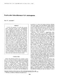
To satisfy both requirements for stability and grid dispersion at those problems, a
P-SV staggered-grid scheme is applied. Note the structure of the elastic wave problem,
eq.(19)-eq.(23),theyallowthestressandparticlevelocitytobespatiallyinterlacedonthe
gridsasinFig. 2. Thestaggered-gridschemeallowsthespatialderivativetobecomputed
to a much higher accuracy (e.g. Levander, 1988). (This computational aspect is similar to
the staggered grid finite difference approach to the Stokes problem, discussed in sec. .)
To add the complexity, the stress and velocity field can also staggered in time. Follow
the explicit scheme,the second order difference equationsfor Equation (19)-(23)are:
u k+1/2
i+1/2,j = uk−1/2
v k+1/2
i,j+1/2 = vk−1/2
i+1/2,j +b i+1/2,j
+b i+1/2,j
∆t
∆h
i,j+1/2 +b i,j+1/2
∆t
( )
Σi+1,j k ∆h
− Σk i,j
(
Γi+1/2,j+1/2 k − Γk i+1/2,j−1/2
∆t
(
∆h
+b i,j+1/2
∆t
∆h
USCGEOL557: ModelingEarth Systems 4
Γi+1/2,j+1/2 k − Γk i−1/2,j+1/2
(
Ξ k i,j+1 − Ξk i,j
)
, (25)
)
)
, (26)

1 WAVEPROPAGATION
Figure2: 2Dstaggeredfinitedifference gridfor wavepropagation.
i,j
= Σi,j k + (λ +2µ) ∆t
i,j
∆h
∆t
+ λ i,j
∆h
Σ k+1
i,j
= Ξi,j k + (λ +2µ) ∆t
i,j
∆h
∆t
+ λ i,j
∆h
Ξ k+1
(
u k+1/2
i+1/2,j −uk+1/2 i−1/2,j
(
v k+1/2
i,j+1/2 −vk+1/2 i,j−1/2
(
v k+1/2
i,j+1/2 −vk+1/2 i,j−1/2
(
u k+1/2
i+1/2,j −vk+1/2 i−1/2,j
Γ k+1
i+1/2,j+1/2 = Γk i+1/2,j+1/2 + µ i+1/2,j+1/2
∆t
(
∆h
+ µ i+1/2,j+1/2
∆t
∆h
To time-evolve the solution for one full ∆t, wefollow:
1. update velocities from the stress;
2. update the stress from the velocities.
For a homogeneous medium, the stability condition is
)
)
, (27)
)
)
, (28)
v k+1/2
i+1,j+1/2 −vk+1/2 i,j+1/2
(
u k+1/2
i+1/2,j+1 −uk+1/2 i+1/2,j
)
)
. (29)
v P
∆t
∆h < 1 √
2
, (30)
USCGEOL557: ModelingEarth Systems 5

1 WAVEPROPAGATION
where
v P =
√
λ +2µ
ρ
(31)
isthe P-wave velocity. Thestability condition isindependentof the S-wave velocity
√ µ
v S =
ρ
(32)
because information will propagate atthe P wavespeed.
To minimize the grid dispersion, the spatial sampling required at least 10 gridpoints
per wavelength, which is defined by the v P . For a 4 th -order approach, the sampling rate
can be reduced to5gridpoints/wavelength (Levander, 1988).
Several other issues are alsovery important in wave propagation in practice:
1. If a boundary condition is not well implemented, the related reflected waves from
the boundaries of the domain will affect the results strongly. Depending on the
problem, different boundary conditions can be applied to the edges: free-surface
conditions,absorbingboundaries(ClaytonandEngquist,1977),andtherecentlywidelyadopted
Perfectly Matched Layer (PML)absorbing boundary (Collinoand Tsogka,
2001).
2. Thesource excitation, which initializesthewavepropagation, alsohastobetreated
with care. In general, a source can be implemented by simply adding a prescribed
source time function to the source mesh. For example, an explosion point source
time function S(t) can be addedto the 2Delastic case as:
τ xx or zz (source grid) = τ xx or zz (FD solution at source grid) +S(t)
1.2.1 Exercise2
• Program the 2D elastic wave propagation in staggered grid scheme as in Fig. 2
(wave_elastic_staggered_2D.m). Choose ∆t and ∆h and describe the wavefield
(both vertical and horizontal components) for the model with uniform velocities.
Identifythe first P and SV arrivalson the recorded seismograms.
• Include a thin liquid layer (v S = 0) in the model and explain the result. Note for a
typical wave propagation problem, the input models are v P , v S , and density ρ, so
the conversions to λ and µ are required in the program.
USCGEOL557: ModelingEarth Systems 6

BIBLIOGRAPHY
Bibliography
Clayton, R., and H. Engquist (1977), Absorbing boundary conditions for acoustic and
elasticwave equations, Bull. Seismol.Soc. Am.,67, 1529–1540.
Collino, F., and C. Tsogka (2001), Application of the perfectly matched absorbing layer
model to the linear elastodynamic problem in anisotropic heterogeneous media, Geophysics,66,294–307.
Levander, A. R. (1988), Fourth-order finite-difference P-SV seismograms, Geophysics, 53,
1425–1436.
USCGEOL557: ModelingEarth Systems 7