the 3D-Dock Manual (PDF) - Structural Bioinformatics Group

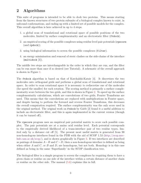
2 Algorithms
This suite of programs is intended to be able to dock two proteins. This means starting
from the known structures of two protein subunits of a biological complex known to exist, in
unbound conformations, and ending up with a limited set of possible models for the complex.
This overall algorithm is here achieved in up to 4 steps.
1. a global scan of translational and rotational space of possible positions of the two
molecules, limited by surface complementarity and an electrostatic filter (ftdock).
2. an empirical scoring of the possible complexes using residue level pair potentials (rpscore
(and rpdock)).
3. using biological information to screen the possible complexes (filter).
4. an energy minimisation and removal of steric clashes on the side-chains of the interface
(multidock [3]).
The middle two steps are interchangeable in the order in which they are run, and the filter
can be run more than once if so desired (see Tutorial). A schematic of the overall approach
is shown in Figure 1.
The ftdock algorithm is based on that of Katchalski-Katzir [4]. It discretises the two
molecules onto orthogonal grids and performs a global scan of translational and rotational
space. In order to scan rotational space it is necessary to rediscretise one of the molecules
(for speed the smaller) for each rotation. The scoring method is primarily a surface complementarity
score between the two grids, and this is shown in Figure 2. To speed up the surface
complementarity calculations, which are convolutions of two grids, Fourier Transforms are
used. This means that the convolutions are replaced with multiplications in Fourier space,
and despite having to perform the forward and reverse Fourier Transforms, this decreases
the overall computation required. The surface complementarity was the only score used in
the original method. The original work on ftdock by Gabb [2] found it a useful addition to
include an electrostatic filter, and this is again implemented in the current version (though
it can be turned off).
The rpscore program uses an empirical pair potential matrix to score each possible complex.
The pair potentials are at a amino acid residue level. Each potential corresponds
to the empirically derived likelihood of a trans-interface pair of two residue types, limited
only by a distance cut off [5]. The present most useful matrix is generated from 90
non-homologous interfaces found in the PDB with the aid of SCOP 1.53 (http://scop.mrclmb.cam.ac.uk/scop/),
and is shown graphically in Figure 3. If two interfaces are described
as pairings of domains A−B and C −D, then a non-homologous interface is defined as being
when either A and C, or B and D, are homologous, but not both. Homology is in this case
defined as being in the same ‘Superfamily’ in the SCOP classification tree.
The biological filter is a simple program to screen the complexes by requiring them to have a
given chain or residue on one side of the interface within a certain distance of another chain
or residue on the other side. The manual (5.6) explains this in full.
3