Chapter 2: Principle of Operation of an Accelerometer

Chapter 2: Principle of Operation of an Accelerometer Page 7
CHAPTER 2
PRINCIPLE OF OPERATION OF AN ACCELEROMETER
In the following work the term ‘accelerometer’ is used to designate the entire transducer,
normally comprising a mechanical sensing element and conversion of the signal from the
mechanical to the electrical domain.
2.1 Derivation of the Motion Equation
The measurement of acceleration always relies on classical Newton’s mechanics. Normally the
acceleration to which a body is subjected is of interest; the accelerometer being rigidly attached
to that body. The transducers which are the subject of this research programme make use of a
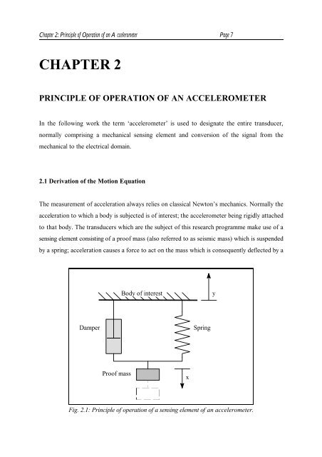
sensing element consisting of a proof mass (also referred to as seismic mass) which is suspended
by a spring; acceleration causes a force to act on the mass which is consequently deflected by a
Body of interest
y
Damper
Spring
Proof mass
x
Fig. 2.1: Principle of operation of a sensing element of an accelerometer.

Chapter 2: Principle of Operation of an Accelerometer Page 8
distance ‘x’as shown in fig. 2.1. Some form of damping is required, otherwise the system would
oscillate at its natural frequency ‘Tn’ for any input signal.
To derive the motion equation of the system, D’Alembert’s principle is applied, where all real
forces acting on the proof mass are equal to the inertia force on the proof mass, Timoshenko and
Young [100]. From the stationary observer’s point of view, the sum of all forces in the y direction
is:
m d 2 y
dt 2
0 ’ &m d 2 (y&x)
dt 2
’ m d 2 x
dt 2
% b dx
dt
% b dx
dt
% kx
% kx ...(2.1)
where:
m: mass of the proof mass,
y: movement of the body of interest,
x: movement of the proof mass,
b: damping factor (assumed to be constant, for this consideration),
k: spring constant.
The second derivative of ‘y’ with respect to time is the acceleration ‘a’ of the body of interest.
2.2 Steady State Performance
In the steady state condition, that is with constant acceleration ‘a’ and constant deflection ‘x’,
eq. (2.1) yields:
ma ’ kx
a ’ kx m
...(2.2)

Chapter 2: Principle of Operation of an Accelerometer Page 9
Here the sensitivity ‘S’ of an accelerometer is defined by:
S ’ x a ’ m k
...(2.3)
2.3 Dynamic Performance
For the dynamic performance it is easier to consider the Laplace transform of eq. (2.1):
x(s)
a(s) ’ 1
s 2 % b m s% k m
...(2.4)
From this equation, the natural frequency ‘Tn’ is
T n
’
k
m
...(2.5)
An upper boundary of the bandwidth of an open loop accelerometer is its natural frequency. It
can be seen by comparing eq. (2.3) and eq. (2.5) that the bandwidth of an accelerometer sensing
element has to be traded off with its sensitivity since S % 1/Tn² (This trade-off can be partly
overcome by applying feedback, which is discussed later).
For the dynamic performance of an accelerometer the damping factor ‘b’ is crucial. For maximum
bandwidth the proof mass should be critically damped; it can be shown that for b = 2mTn this is
the case. It should be noted here that in micromachined accelerometers the damping originates
from the movement of the proof mass in a viscous medium. However, depending on the
mechanical design, the damping coefficient ‘b’cannot be assumed to be constant; this phenomena
will be discussed in sec. 5.3.

Chapter 2: Principle of Operation of an Accelerometer Page 10
2.4 Closed Loop Accelerometer
The accelerometer discussed above, in which the deflection of the proof mass provides a measure
for the acceleration, is commonly referred to as an open loop accelerometer. High performance
transducers have traditionally made use of some form of feedback where an external force is used
to compensate the inertia force on the proof mass due to the acceleration, thus keeping the proof
mass at zero deflection (x = 0). This can be approximately achieved by a closed loop structure
depicted in fig. 2.2
Accelerating
force
F=ma
-
Error
signal
Sensing element of
the accelerometer
x6V
Compensation
Output
signal
Feedback force
Ff
Ff 7 V
Fig. 2.2: Closed loop accelerometer.
The external force has to be derived by a residual deflection of the proof mass. The position of
the proof mass is sensed and converted into a voltage, providing the output signal. The same
voltage is used to generate a feedback force on the proof mass opposing the accelerating input
force. Consequently, the proof mass is only being deflected by the difference between these two
forces which can be considered as the error signal. Some sort of compensation may be required
to ensure the stability of the loop.
In a closed loop accelerometer the sensitivity ‘S’is not inversely proportional to the square of the

Chapter 2: Principle of Operation of an Accelerometer Page 11
natural frequency ‘Tn’ of the sensing element but depends on the loop gain and the form of
compensation. Another advantage is that possible nonlinearities of spring and the damping are
reduced considerably if the proof mass stays at or close to its rest position. Furthermore the
bandwidth of the accelerometer can be increased past the natural frequency of the sensing
element.
In conventional, closed loop accelerometers the feedback force is commonly generated by using
electro-magnetic forces, Sundstrand data sheet [97]. However, in micromachined devices the
dimensions are so small that electrostatic forces can be used to provide the feedback. This has the
advantage of lower power consumption and overcomes the problems of manufacturing
micromachined inductors, Ward and King [109]. At the present time no micromachined
accelerometer is described in the literature that uses electro-magnetic feedback or reset. The
drawback of electrostatic feedback with the proof at a defined potential is that the forces are
proportional to the square of the voltage, hence they are always positive and consequently
negative feedback is difficult to generate. For this reason the feedback relationship is nonlinear.
These problems are discussed in detail in chapter 6.