Observer design by pole placement
Observer design by pole placement
Observer design by pole placement

You also want an ePaper? Increase the reach of your titles
YUMPU automatically turns print PDFs into web optimized ePapers that Google loves.
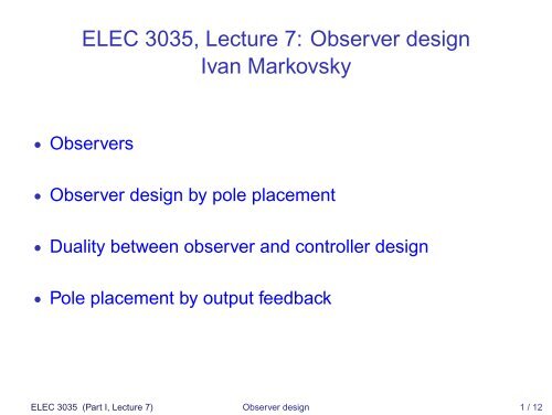
ELEC 3035, Lecture 7: <strong>Observer</strong> <strong>design</strong><br />
Ivan Markovsky<br />
• <strong>Observer</strong>s<br />
• <strong>Observer</strong> <strong>design</strong> <strong>by</strong> <strong>pole</strong> <strong>placement</strong><br />
• Duality between observer and controller <strong>design</strong><br />
• Pole <strong>placement</strong> <strong>by</strong> output feedback<br />
ELEC 3035 (Part I, Lecture 7) <strong>Observer</strong> <strong>design</strong> 1 / 12
General observer <strong>design</strong> problem<br />
Given dynamical system B ext with two types of external variables:<br />
• observed variables w<br />
• to-be-estimated variables z<br />
B ext<br />
w<br />
z<br />
find system (called observer) accepting w and producing z<br />
w<br />
<strong>Observer</strong><br />
z<br />
We will consider the case: B = B i/s/o (A,B,C,D), w = (u,y), z = x.<br />
Lecture 6: nonrecursive, feedforward observer for the initial state x(0)<br />
Now our goal is recursive feedback observer for the current state x(t)<br />
ELEC 3035 (Part I, Lecture 7) <strong>Observer</strong> <strong>design</strong> 2 / 12
Output feedback control<br />
separation and certainty principles<br />
We can extend a given state-feedback controller<br />
to output feedback controller<br />
u = Kx<br />
u = K̂x<br />
<strong>by</strong> using the observer state estimate ̂x in place of x.<br />
u<br />
Plant<br />
y<br />
K<br />
̂x<br />
<strong>Observer</strong><br />
Output feedback controller<br />
ELEC 3035 (Part I, Lecture 7) <strong>Observer</strong> <strong>design</strong> 3 / 12
Internal model and feedback principles<br />
The observer <strong>design</strong> is based on the following principles:<br />
1. Internal model: the model run <strong>by</strong> u, gives an estimate ̂x for x<br />
2. Feedback: correct the estimate ̂x, so that the error<br />
x(t) −̂x(t) =: e(t) → 0 as t → ∞<br />
Let the feedback be a linear function of the output error<br />
feedback correction = L(y − ŷ)<br />
Then the observer for the model B i/s/o (A,B,C,D) is<br />
σ̂x = Âx + Bu − L(y − ŷ)<br />
ŷ = Ĉx + Du<br />
ELEC 3035 (Part I, Lecture 7) <strong>Observer</strong> <strong>design</strong> 4 / 12
Error dynamics<br />
Our goal is to choose L, so that the state error e(t) → 0 as t → ∞.<br />
The dynamics of e is<br />
σe = σ(x −̂x)<br />
= Ax + Bu − Âx − Bu + L(y − ŷ)<br />
= A(x −̂x)+LC(x −̂x)<br />
= (A+LC) e<br />
} {{ }<br />
A o<br />
i.e., e ∈ B ss (A o ) — an autonomous LTI system.<br />
Therefore, e(t) → 0 as t → ∞ is equivalent to stability of B ss (A o ).<br />
ELEC 3035 (Part I, Lecture 7) <strong>Observer</strong> <strong>design</strong> 5 / 12
Comparison with state-feedback stabilization<br />
In the state feedback stabilization problem we have<br />
σx = Ax + Bu and u = Kx<br />
which gives an autonomous LTI closed loop system<br />
σx = (A+BK) x<br />
} {{ }<br />
A c<br />
and the aim is to choose K , so that B ss (A c ) is stable.<br />
ELEC 3035 (Part I, Lecture 7) <strong>Observer</strong> <strong>design</strong> 6 / 12
<strong>Observer</strong> <strong>design</strong> <strong>by</strong> <strong>pole</strong> <strong>placement</strong><br />
The condition e(t) → 0 as t → ∞ is a minimum requirement.<br />
In fact we want e(t) → 0 fast<br />
(possibly in a finite (small) number of steps deadbeat observer)<br />
The error dynamics is governed <strong>by</strong> the <strong>pole</strong>s of the matrix<br />
A o := A+LC<br />
so for desired error dynamics we can<br />
select desired <strong>pole</strong> locations of A o and choose L to achieve them.<br />
ELEC 3035 (Part I, Lecture 7) <strong>Observer</strong> <strong>design</strong> 7 / 12
Duality of the observer PP and controller PP problems<br />
<strong>Observer</strong> PP problem: Choose L, so that<br />
det ( zI −(A+LC) ) = p des (z)<br />
Controller PP problem: Choose K , so that<br />
det ( zI −(A+BK) ) = p des (z)<br />
<strong>Observer</strong> PP is not a new problem:<br />
det ( zI −(A+LC) ) ( (zI ) ) ⊤<br />
= det −(A+LC)<br />
(<br />
)<br />
= det zI −(A ⊤ + C ⊤ L ⊤ )<br />
( )<br />
= det zI −(Ã+ ˜B ˜K)<br />
=⇒ observer PP is controller PP for the dual system.<br />
ELEC 3035 (Part I, Lecture 7) <strong>Observer</strong> <strong>design</strong> 8 / 12
The results for state feedback PP can be restated for observer PP:<br />
Theorem:<br />
The eigenvalues of A+LC can be assigned choosing L<br />
to any locations in C if and only if A,C is observable.<br />
<strong>Observer</strong> canonical form ↔ Controller canonical form<br />
Lemma:<br />
• Let A,c and A ′ ,c ′ be two observable pairs and<br />
• assume that A and A ′ have the same char. polynomials.<br />
Then there is a unique similarity transformation given <strong>by</strong> the matrix<br />
T := ( O(A ′ ,c ′ ) ) −1 O(A,c)<br />
such that<br />
T −1 AT = A ′ and cT = c ′ .<br />
ELEC 3035 (Part I, Lecture 7) <strong>Observer</strong> <strong>design</strong> 9 / 12
Closed-loop system with output feedback controller<br />
Consider the closed loop system<br />
u<br />
Plant<br />
y<br />
K<br />
̂x<br />
<strong>Observer</strong><br />
Output feedback controller<br />
where<br />
Plant: σx = Ax + Bu, y = Cx + Du<br />
<strong>Observer</strong>:<br />
State feedback controller:<br />
σ̂x = Âx + Bu − L(y − Ĉx − Du)<br />
u = K̂x<br />
ELEC 3035 (Part I, Lecture 7) <strong>Observer</strong> <strong>design</strong> 10 / 12
Feedback controller:<br />
σ̂x = (A+LC)̂x +(B + LD)u − Ly,<br />
= (A+LC + BK + LDK)̂x − Ly<br />
u = K̂x<br />
Note: the feedback controller is a dynamical system<br />
Closed-loop system:<br />
[ [ ]<br />
x̂x] A BK<br />
σ =<br />
−LC A+LC + BK][ x̂x<br />
Note: closed-loop system order = plant order + controller order<br />
Error equation:<br />
[ [ ]<br />
x A+BK −BK x<br />
σ =<br />
e]<br />
0 A+LC][<br />
e<br />
ELEC 3035 (Part I, Lecture 7) <strong>Observer</strong> <strong>design</strong> 11 / 12
Example: output feedback deadbeat control<br />
−2<br />
−3<br />
−4<br />
1 x 10⁵ 0<br />
t<br />
1<br />
−1<br />
0<br />
y<br />
−1<br />
−2<br />
5 10 15 20<br />
−3<br />
2 x 10⁵ t<br />
u<br />
5 10 15 20<br />
15th order single-input open-loop system, 30 order closed-loop system<br />
(The same system as the one used in the example of Lecture 1)<br />
ELEC 3035 (Part I, Lecture 7) <strong>Observer</strong> <strong>design</strong> 12 / 12