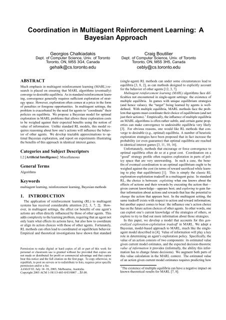
Coordination in Multiagent Reinforcement Learning: A Bayesian ...

the repeated game itself. 5 Standard Bayesian updating methods areused to maintain these beliefs over time, and best responses areplayed by the agent w.r.t. the expectation over strategy profiles.Repeated games are a special case of stochastic games [15, 5],which can be viewed as a multiagent extension of MDPs. Formally,a stochastic game G = 〈α, {A i} i∈α, S,Pr, {R i} i∈α〉 consists offive components. The agents α and action sets A i are as in a typicalgame, and the components S and Pr are as in an MDP, exceptthat Pr now refers to joint actions a ∈ A = ×A i. R i is athe reward function for agent i, defined over states s ∈ S (pairs〈s, a〉 ∈ S × A). The aim of each agent is, as with an MDP, toact to maximize the expected sum of discounted rewards. However,the presence of other agents requires treating this problem ina game theoretic fashion. For particular classes of games, such aszero-sum stochastic games [15, 5], algorithms like value iterationcan be used to compute Markovian equilibrium strategies.The existence of multiple “stage game” equilibria is again a problemthat plagues the construction of optimal strategies for stochasticgames. Consider another simple identical interest example, thestochastic game shown in Figure 3(a). In this game, there are twooptimal strategy profiles that maximize reward. In both, the firstagent chooses to “opt in” at state s 1 by choosing action a, whichtakes the agents (with high probability) to state s 2; then at s 2 bothagents either choose a or both choose b—either joint strategy givesan optimal equilibrium.Intuitively, the existence of these two equilibria gives rise to acoordination problem at state s 2. If the agents choose their partof the equilibrium randomly, there is a 0.5 chance that they miscoordinateat s 2, thereby obtaining an expected immediate rewardof 0. On this basis, one might be tempted to propose methodswhereby the agents decide to “opt out” at s 1 (the first agent takesaction b) and obtain the safe payoff of 6. However, if we allowsome means of coordination—for example, simple learning ruleslike fictitious play or randomization—the sequential nature of thisproblem means that the short-term risk of miscoordination at s 2 canbe more than compensated for by the eventual stream of high payoffsshould they coordinate. Boutilier [1] argues that the solutionof games like this, assuming some (generally, history-dependent)mechanism for resolving these stage game coordination problems,requires explicit reasoning about the odds and benefits of coordination,the expected cost of attempting to coordinate, and the alternativecourses of action.Repeated games can be viewed as stochastic games with a singlestate. If our concern is not with stage-game equilibrium, but withreward accrued over the sequence of interactions, techniques forsolving stochastic games can be applied to solving such repeatedgames. Furthermore, the points made above regarding the risksassociated with using specific learning rules for coordination canbe applied with equal force to repeated games.2.3 Multiagent RLIn this section, we describe some existing approaches to MARL,and point out recent efforts to augment standard RL schemes to encourageRL agents in multiagent systems to converge to optimalequilibria. Intuitively, MARL can be viewed as the direct or indirectapplication of RL techniques to stochastic games in whichthe underlying model (i.e., transitions and rewards) are unknown.In some cases, it is assumed that the learner is even unaware (orchooses to ignore) the existence of other agents.Formally, we suppose we have some underlying stochastic game5 A strategy in the repeated game is any mapping from the observedhistory of play to a (stochastic) action choice. This admits the possibilityof modeling other agents’s learning processes.G = 〈α, {A i} i∈α, S,Pr, {R i} i∈α〉. We consider the case whereeach agent knows the “structure” of the games—that is, it knowsthe set of agents, the actions available to each agent, and the set ofstates—but knows neither the dynamics Pr, nor the reward functionsR i. The agents learn how to act in the world through experience.At each point in time, the agents are at a known state s,and each agent i executes one of its actions; the resulting joint actiona induces a transition to state t and a reward r i for each agent.We assume that each agent can observe the actions chosen by otheragents, the resulting state t, and the rewards r i.Littman [12] devised an extension of Q-learning for zero-sumMarkov games called minimax-Q. At each state, the agents haveestimated Q-values over joint actions, which can be used to computean (estimated) equilibrium value at that state. Minimax-Q convergesto the equilibrium value of the stochastic game [13]. Huand Wellman [7] apply similar ideas—using an equilibrium computationon estimated Q-values to estimate state values—to generalsum games, with somewhat weaker convergence guarantees. Algorithmshave also been devised for agents that do not observe thebehavior of their counterparts [2, 8].Identical interest games have drawn much attention, providingsuitable models for task distribution among teams of agents. Clausand Boutilier [3] proposed several MARL methods for repeatedgames in this context. A simple joint-action learner (JAL) protocollearned the (myopic, or one-stage) Q-values of joint actions.The novelty of this approach lies in its exploration strategy: (a)a fictitious play protocol estimates the strategies of other agents;and (b) exploration is biased by the expected Q-value of actions.Specifically, the estimated value of an action is given by its expectedQ-value, where the expectation is taken w.r.t. the fictitiousplay beliefs over the other agents’s strategies. When semi-greedyexploration is used, this method will converge to an equilibrium inthe underlying stage game.One drawback of the JAL method is the fact that the equilibriumit converges to depends on the specific path of play, whichis stochastic. Certain equilibria can exhibit serious resistance—forexample, the odds of converging to an optimal equilibrium in thepenalty game above are quite small (and decrease dramatically withthe magnitude of the penalty). Claus and Boutilier propose severalheuristic methods that bias exploration toward optimal equilibria:for instance, action selection can be biased toward actions that formpart of an optimal equilibrium. In the penalty game, for instance,despite the fact that agent B may be predicted to play a strategythat makes the a0 look unpromising, the repeated play of the a0by A can be justified by optimistically assuming B will play itspart of this optimal equilibrium. This is further motivated by thefact that repeated play of a0 would eventually draw B toward thisequilibrium.This issue of learning optimal equilibria in identical interest gameshas been addressed recently in much greater detail. Lauer andRiedmiller [11] describe a Q-learning method for identical intereststochastic games that explicitly embodies this optimistic assumptionin its Q-value estimates. Kapetanakis and Kudenko [10] proposea method called FMQ for repeated games that uses the optimisticassumption to bias exploration, much like [3], but in the contextof individual learners. Wang and Sandholm [16] similarly usethe optimistic assumption in repeated games to guarantee convergenceto an optimal equilibrium. We critique these methods below.3. A BAYESIAN VIEW OF MARLThe spate of activity described above on MARL in identical interestgames has focused exclusively on devising methods that ensureeventual convergence to optimal equilibria. In cooperative

games, this pursuit is well-defined, and in some circumstances maybe justified. However, these methods do not account for the factthat—by forcing agents to undertake actions that have potentiallydrastic effects in order to reach an optimal equilibrium—they canhave a dramatic impact on accumulated reward. The penalty gamewas devised to show that these highly penalized states can bias(supposedly rational) agents away from certain equilibria; yet optimisticexploration methods ignore this and blindly pursue theseequilibria at all costs. Under certain performance metrics (e.g., averagereward over an infinite horizon) one might justify these techniques.6 However, using the discounted reward criterion (which allof these methods are designed for), the tradeoff between long-termbenefit and short-term cost should be addressed.This tradeoff was discussed above in the context of known-modelstochastic games. In this section, we attempt to address the sametradeoff in the RL context. To do so, we formulate a Bayesianapproach to model-based MARL. By maintaining probabilistic beliefsover the space of models and the space of opponent strategies,our learning agents can explicitly account for the effects their actionscan have on (a) their knowledge of the underlying model; (b)their knowledge of the other agent strategies; (c) expected immediatereward; and (d) expected future behavior of other agents. Components(a) and (c) are classical parts of the single-agent BayesianRL model [4]. Components (b) and (d) are key to the multiagentextension, allowing an agent to explicitly reason about the potentialcosts and benefits of coordination.3.1 Theoretical UnderpinningsWe assume a stochastic game G in which each agent knows thegame structure, but not the reward or transition models. A learningagent i is able to observe the actions taken by all agents, the resultinggame state, and the rewards received by other agents. Thusan agent’s experience at each point in time is simply 〈s, a,r i, t〉,where s is a state in which joint action a was taken, r i is the rewardreceived, and t is the resulting state.A Bayesian MARL agent has some prior distribution over thespace of possible models as well as the space of possible strategiesbeing employed by other agents. These beliefs are updatedas the agent acts and observes the results of its actions and the actionchoices of other agents. The strategies of other agents may behistory-dependent, and we allow our Bayesian agent (BA) to assignpositive support to such strategies. As such, in order to make accuratepredictions about the actions others will take, the BA mustmonitor appropriate observable history. In general, the history (orsummary thereof) required will be a function of the strategies towhich the BA assigns positive support. We assume that the BAkeeps track of sufficient history to make such predictions. 7The belief state of the BA has the form b = 〈P M, P S, s, h〉,where: P M is some density over the space of possible models (i.e.,games); P S is a joint density over the possible strategies playedby other agents; s is the current state of the system; and h is asummary of the relevant aspects of game history, sufficient to predictthe action of any agent given any strategy consistent with P S.Given experience 〈s, a, r i, t〉, the BA updates its belief state usingstandard Bayesian methods. The updated belief state is:b ′ = b(〈s, a,r i, t〉) = 〈P ′ M, P ′ S, t, h ′ 〉 (2)6 Even then, more refined measures such as bias optimality mightcast these techniques in a less favorable light.7 For example, should the BA believe that its opponent’s strategylies in the space of finite state controller that depends on the lasttwo joint actions played, the BA will need to keep track of these lasttwo actions. If it uses fictitious play beliefs (which can be viewedas Dirichlet priors) over strategies, no history need be maintained.Updates are given by Bayes rule: P M(m) ′ = z Pr(t,r i|a, m)P M(m)and P S(σ ′ −i) = z Pr(a −i|s, h, σ −i)P S(σ −i). And h ′ is a suitableupdate of the observed history (as described above). Thismodel combines aspects of Bayesian reinforcement learning [4]and Bayesian strategy modeling [9].To make belief state maintenance tractable (and admit computationallyviable methods for action selection below), we assumea specific form for these beliefs [4]. First, our prior over modelswill be factored into independent local models for both rewardsand transitions. We assume independent priors PR s over reward distributionsat each state s, and P s,aDover system dynamics for eachstate and joint action pair. These local densities are Dirichlet, whichare conjugate for the multinomial distributions to be learned. Thismeans that each density can be represented using a small numberof hyperparameters, expected transition probabilities can be computedreadily, and the density can be updated easily. For example,our BA’s prior beliefs about the transition probabilities for jointaction a at state s will be represented by a vector n s,a with oneparameter per successor state t. Expected transition probabilitiesand updates of these beliefs are as described in Section 2.1. Theindependence of these local densities is assured after each update.Second, we assume that the beliefs about opponent strategies canbe factored and represented in some convenient form. For example,it would be natural to assume that the strategies of other agentsare independent. Simple fictitious play models could be used tomodel the BA’s beliefs about opponent strategies (corresponding toDirichlet priors over mixed strategies), allowing ready update andcomputation of expectations, and obviating the need to store historyin the belief state. Similarly, distributions over specific classes offinite state controllers could also be used. We will not pursue furtherdevelopment of such models in this paper, since we use onlysimple opponent models in our experiments below. But the developmentof tractable classes of (realistic) opponent models remainsan interesting problem.We provide a different perspective on Bayesian exploration thanthat described in [4]. The value of performing an action a i at abelief state b can be viewed as involving two main components: anexpected value with respect to the current belief state; and its impacton the current belief state. The first component is typical inRL, while the second captures the expected value of information(EVOI) of an action. Since each action gives rise to some “response”by the environment that changes the agent’s beliefs, andthese changes in belief can influence subsequent action choice andexpected reward, we wish to quantify the value of that informationby determining its impact on subsequent decisions.EVOI need not be computed directly, but can be combined with“object-level” expected value through the following Bellman equationsover the belief state MDP:Q(a i, b) = X a −iPr(a −i|b) X tXPr(t|a i ◦ a −i, b)r iPr(r i|a i ◦ a −i, b)[r i + γV (b(〈s,a, r i, t〉))] (3)V (b) = maxa iQ(a i, b) (4)These equations describe the solution to the POMDP that representsthe exploration-exploitation problem, by conversion to a beliefstate MDP. These can (in principle) be solved using any methodfor solving high-dimensional continuous MDPs—of course, in practice,a number of computational shortcuts and approximations willbe required (as we detail below). We complete the specification

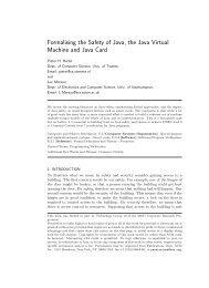
80155060100-5040200-20BVPIBOLWoLFCombined Boltzmann ExplorationOptimistic Boltzmann ExplorationKK50-5BVPIBOLWoLFCombined Boltzmann ExplorationOptimistic Boltzmann ExplorationKK-100-150-200-250-300BVPIBOLWoLFCombined Boltzmann ExplorationOptimistic Boltzmann ExplorationKKBVPI (uninf. priors, penalty=-100)BOL (uninf. priors, penalty=-100)-40-10-350-400-600 20 40 60 80 100Number of Iterations(a) k = −20, γ = 0.95, uninf. priors-150 5 10 15 20 25 30 35 40 45 50Number of Iterations(b) k = −20, γ = 0.75, uninf. priors-4500 20 40 60 80 100Number of Iterations(c) k = −100, γ = 0.95, inform. priorsFigure 1: Penalty Game Resultswith the straightforward definition of the following terms:ZPr(a −i|b) = Pr(a −i|σ −i)P S(σ −i) (5)σ −iZPr(t|a, b) = Pr(t|s, a, m)P M(m) (6)mZPr(r i|b) = Pr(r i|s, m)P M(m) (7)mWe note that the evaluation of Eqs. 6 and 7 is trivial using the decomposedDirichlet priors mentioned above.This formulation determines the optimal policy as a function ofthe BA’s belief state. This policy incorporates the tradeoffs betweenexploration and exploitation, both with respect to the underlying(dynamics and reward) model, and with respect to the behaviorof other agents. As with Bayesian RL and Bayesian learning ingames, no explicit exploration actions are required. Of course, it isimportant to realize that this model may not converge to an optimalpolicy for the true underlying stochastic game. Priors that fail toreflect the true model, or unfortunate samples early on, can easilymislead an agent. But it is precisely this behavior that allows anagent to learn how to behave well without drastic penalty.3.2 Computational ApproximationsSolving the belief state MDP above will generally be computationallyinfeasible. In specific MARL problems, the generality ofsuch a solution—defining as it does a value for every possible beliefstate—is not needed anyway. Most belief states are not reachablegiven a specific initial belief state. A more directed search-basedmethod can be used to solve this MDP for the agent’s current beliefstate b. We consider a form of myopic EVOI in which only immediatesuccessor belief states are considered, and their values areestimated without using VOI or lookahead.Formally, myopic action selection is defined as follows. Givenbelief state b, the myopic Q-function for each a i ∈ A i is:Q m(a i, b) = X a −iPr(a −i|b) X tXPr(t|a i ◦ a −i, b)Pr(r i|a i ◦ a −i, b)[r + γV m(b(〈s,a, r i, t〉))] (8)r iZV m(b) = max Q(a i, s|m, σ −i)P M(m)P S(σ −i) (9)a iZm σ −iThe action performed is that with maximum myopic Q-value. Eq. 8differs from Eq. 3 in the use of the myopic value function V m,which is defined as the expected value of the optimal action at thecurrent state, assuming a fixed distribution over models and strategies.8 Intuitively, this myopic approximation performs one steplookaheadin belief space, then evaluates these successor states bydetermining the expected value to BA w.r.t. a fixed distribution overmodels, and a fixed distribution over successor states.This computation involves the evaluation of a finite number ofsuccessor belief states—A · R · S such states, where A is the numberof joint actions, R is the number of rewards, and S is the sizeof the state space (unless b restricts the number of reachable states,plausible strategies, etc.). Greater accuracy can be realized withmultistage lookahead, with the requisite increase in computationalcost. Conversely, the myopic action can be approximated by samplingsuccessor beliefs (using the induced distributions defined inEqs. 5, 6, 7) if the branching factor A · R · S is problematic.The final bottleneck involves the evaluation of the myopic valuefunction V m(b) over successor belief states. The Q(a i, s|m, σ −i)terms are Q-values for standard MDPs, and can be evaluated usingstandard methods, but direct evaluation of the integral over allmodels is generally impossible. However, sampling techniques canbe used [4]. Specifically, some number of models can be sampled,the corresponding MDPs solved, and the expected Q-values estimatedby averaging over the sampled results. Various techniquesfor making this process more efficient can be used as well, includingimportance sampling (allowing results from one MDP to beused multiple times by reweighting) and “repair” of the solutionfor one MDP when solving a related MDP [4].For certain classes of problems, this evaluation can be performeddirectly. For instance, suppose a repeated game is being learned,and the BA’s strategy model consists of fictitious play beliefs. Theimmediate expected reward of any action a i taken by the BA (w.r.t.successor b ′ ) is given by its expectation w.r.t. its estimated rewarddistribution and fictitious play beliefs. The maximizing action a ∗ iwith highest immediate reward will be the best action at all subsequentstages of the repeated game—and has a fixed expected rewardr(a ∗ i ) under the myopic (value) assumption that beliefs are fixed byb ′ . Thus the long-term value at b ′ is r(a ∗ i )/(1 − γ).The approaches above are motivated by approximating the directmyopic solution to the “exploration POMDP.” A different approachto this approximation is proposed in [4], which estimates the (myopic)value of obtaining perfect information about Q(a,s). Supposethat, given an agent’s current belief state, the expected value8 We note that V m(b) only provides a crude measure of the valueof belief state b under this fixed uncertainty. Other measures couldinclude the expected value of V (s|m, σ −i).

3.514031202.510021.58060BVPIWoLFa a; 0s1s2a a; 0s3a a; 0s4a a; 0a a; 10s510.5BVPIWoLF4020b b; 2 b b; 2 b b; 2 b b; 2(a) Chain World Domain00 5 10 15 20 25 30 35 40 45 50Number of Iterations(b) γ = 0.7500 20 40 60 80 100 120 140 160Number of Iterations(c) γ = 0.99Figure 2: Chain World Resultsof action a is given by Q(a, s). Let a 1 be the action with highestexpected Q-value and state s and a 2 be the second-highest. We definethe gain associated with learning that the true value of Q(a,s)(for any a) is in fact q as follows:8 Q(a 1, s)0, otherwiseIntuitively, the gain reflects the effect on decision quality of learningthe true Q-value of a specific action at state s. In the first twocases, what is learned causes us to change our decision (in the firstcase, the estimated optimal action is learned to be worse than predicted,and in the second, some other action is learned to be optimal).In the third case, no change in decision at s is induced, so theinformation has no impact on decision quality.Adapted to our setting, a computational approximation to thisnaive sampling approach involves the following steps:(a) a finite set of k models is sampled from the density P M;(b) each sampled MDP j is solved (w.r.t. the density P S over strategies),giving optimal Q-values Q j (a i, s) for each a i in thatMDP, and average Q-value Q(a i, s) (over all k MDPs);(c) for each a i, compute gain s,ai (Q j (a i, s)) for each of the kMDPS; let EVPI(a i, s) be the average of these k values;(d) define the value of a i to be Q(a i, s)+EVPI(a i, s) and executethe action with highest value.This approach can benefit from the use of importance sampling andrepair (with minor modifications). Naive sampling can be morecomputationally effective than one-step lookahead (which requiressampling and solving MDPs from multiple belief states). The pricepaid is approximation inherent in the perfect information assumption:the execution of joint action a does not come close to providingperfect information about Q(a,s).4. EXPERIMENTAL RESULTSWe have conducted a number of experiments with both repeatedand stochastic games to evaluate the Bayesian approach. We focuson two-player identical interest games largely to compare to existingmethods for “encouraging” convergence to optimal equilibria.The Bayesian methods examined are one-step lookahead (BOL)and naive sampling for estimating VPI (BVPI) described in Section3. In all cases, the Bayesian agents use a simple fictitious playmodel to represent their uncertainty over the other agent’s strategy.Thus at each iteration, a BA believes its opponent to play an actionwith the empirical probability observed in the past (for multistategames, these beliefs are independent at each state).BOL is used only for repeated games, since these allow the immediatecomputation of expected values over the infinite horizonat the successor belief states: expected reward for each joint actioncan readily be combined with the BA’s fictitious play beliefs tocompute the expected value of an action (over the infinite horizon)since the only model uncertainty is in the reward. BVPI is usedfor both repeated and multi-state games. In all cases, five modelsare sampled to estimate the VPI of the agent’s actions. The strategypriors for the BAs are given by Dirichlet parameters (“priorcounts”) of 0.1 or 1 for each opponent action. The model priors aresimilarly uninformative, with each state-action pair given the sameprior distribution over reward and transition distributions (exceptfor one experiment as noted).We first compare our method to several different algorithms on astochastic version of the penalty game described above. The gameis altered so that joint actions provide a stochastic reward, whosemean is the value shown in the game matrix. 9 We compare theBayesian approach to the following algorithms. KK is an algorithm[10] that biases exploration to encourage convergence to optimalequilibria in just these types of games. Two related heuristic algorithmsthat also bias exploration optimistically are the OptimisticBoltzmann (OB) and Combined OB (CB) [3] are also evaluated.Unlike KK, these algorithms observe and make predictions aboutthe other agent’s play. Finally, we test the more general algorithmWoLF-PHC [2], which works with arbitrary, general-sum stochasticgames (and has no special heuristics for equilibrium selection).In each case the game is played by two learning agents of the sametype. The parameters of all algorithms were empirically tuned togive good performance.The first set of experiments tested these agents on the stochasticpenalty game with k set to −20 and discount factors of 0.95 and0.75. Both BOL and BVPI agents use uninformative priors overthe set of reward values. 10 Results appear in in Figures 1(a) and (b)showing the total discounted reward accumulated by the learningagents, averaged over 30 trials. Discounted accumulated rewardprovides a suitable way to measure both the cost being paid in theattempt to coordinate as well as the benefits of coordination (or lack9 Each joint action gives rise to X distinct rewards.10 Specifically, any possible reward (for any joint action) is givenequal (expected) probability in the agent’s Dirichlet priors.

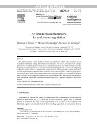
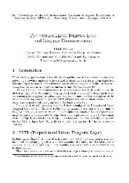
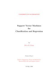
620018051604140120s1* *s4a,a; b,bs2a,b; b,aa *b ** *s5s3* *s6* *+10-10+632100 5 10 15 20 25 30 35 40 45 50Number of IterationsBVPIWoLF100806040200-200 20 40 60 80 100 120 140 160Number of IterationsBVPIWoLF(a) The Opt In or Out Domain(b) γ = 0.75(c) γ = 0.99Figure 3: “Opt In or Out” Results: Low Noisethereof). The results show that both Bayesian methods perform significantlybetter than the methods designed to force convergence toan optimal equilibrium. Indeed, OB, CB and KK converge to anoptimal equilibrium in virtually all of their 30 runs, but clearly paya high price. 11 By comparison, when γ = 0.95, the ratio of convergenceto an optimal equilibrium, the nonoptimal equilibrium, ora nonequilibrium is, for BVPI 25/1/4 and for BOL 14/16/0. Surprisingly,WoLF-PHC does better than OB, CB and KK in bothtests. In fact, this method outperforms the BVPI agent in the caseof γ = 0.75 (largely because BVPI converges to a nonequilibrium5 times and the suboptimal equilibrium 4 times). WoLF-PHC convergesin each instance to an optimal equilibrium.We repeated this comparison on a more “difficult” problem witha mean penalty of -100 (and increasing the variance of the rewardfor each action). To test one of the benefits of the Bayesian perspectivewe included a version of BOL and BVPI with informativepriors (giving it strong information about rewards by restricting theprior to assign (uniform) nonzero expected probability to the smallrange of truly feasible rewards for each action). Results are shownin Figure 1(c) (averaged over 30 runs). Wolf-PHC and CB convergeto the optimal equilibrium each time, while the increased rewardstochasticity made it impossible for KK and OB to convergeat all. All four methods perform poorly w.r.t. discounted reward.The Bayesian methods perform much better. Not surprisingly, theagents BOL and BVPI with informative priors do better than their“uninformed” counterparts; however, because of the high penalty(despite the high discount factor), they converge to the suboptimalequilibrium most of the time (22 and 23 times, respectively).We also applied the Bayesian approach to two identical-interest,multi-state, stochastic games. The first is a version of Chain World[4] modified for multiagent coordination, and is illustrated in Figure2(a). The optimal joint policy is for the agents to do action aat each state, though these actions have no payoff until state s 5 isreached. Coordinating on b leads to an immediate, but smaller, payoff,and resets the process. 12 Unmatched actions 〈a,b〉 and 〈b, a〉result in zero-reward self-transitions (omitted from the diagram forclarity). Transitions are noisy, with a 10% chance that an agent’saction has the “effect” of the opposite action. The original ChainWorld is difficult for standard RL algorithms, and is made especiallydifficult here by the requirement of coordination.We compared BVPI to WoLF-PHC on this domain using two11 All penalty game experiments were run to 500 games, though onlythe interesting initial segments of the graphs are shown.12 As above, rewards are stochastic with means shown in the figure.different discount factors, plotting the total discounted reward (averagedover 30 runs) in Figure 2(b) and (c). Only initial segmentsare shown, though the results project smoothly to 50000 iterations.BVPI compares favorably to Wolf-PHC in terms of online performance.BVPI converged to the optimal policy in 7 (of 30) runswith γ = 0.99 and in 3 runs with γ = 0.75, intuitively reflectingthe increased risk aversion due to increased discounting. WoLF-PHC rarely even managed to reach state s 5, though in 2 (of 30)runs with γ = 0.75 it stumbled across s 5 early enough to convergeto the optimal policy. The Bayesian approach manages to encourageintelligent exploration of action space in a way that trades offrisks and predicted rewards; and we see increased exploration withthe higher discount factor, as expected.The second multi-state game is “Opt in or Out” shown in Figure3(a). The transitions are stochastic, with the action selectedby an agent having the “effect” of the opposite action with someprobability. Two versions of the problem were tested, one with low“noise” (probability 0.05 of an action effect being reversed), andone with “medium” noise level (probability roughly 0.11). Withlow noise, the optimal policy is as if the domain were deterministic(the first agent opts in at s 1 and both play a coordinated choiceat s 2), while with medium noise, the “opt in” policy and the “optout” policy (where the safe move to s 6 is adopted) have roughlyequal value. BVPI is compared to WoLF-PHC under two differentdiscount rates, with low noise results shown in Figure 3(b) and(c), and high noise results in Figure 4(a) and (b). Again BVPIcompares favorably to WoLF-PHC, in terms of dicounted rewardaveraged over 30 runs. In the low noise problem, BVPI convergedto the optimal policy in 18 (of 30) runs with γ = 0.99 and 15 runswith γ = 0.75. The WoLF agents converged in the optimal policyonly once with γ = 0.99, but 17 times with γ = 0.75. Withmedium noise, BVPI chose the “opt in” policy in 10 (0.99) and13 (0.75) runs, but learned to coordinate at s 2 even in the “opt out”cases. Interestingly, WoLF-PHC always converged on the “opt out”policy (recall both policies are optimal with medium noise).Finally, we remark that the Bayesian methods do incur greatercomputational cost per experience than the simpler model-free RLmethods we compared to. BOL in particular can be intensive, takingup to 25 times as long to select actions in the repeated gameexperiments as BVPI. Still, BOL computation time per step is onlyhalf a millisecond. BVPI is comparable to all other methods on repeatedgames. In the stochastic games, BVPI takes roughly 0.15msto compute action selection, about 8 times as long as WoLF inChainWorld, and 24 times in Opt In or Out.

4.543.532.521.510.50-0.50 5 10 15 20 25 30 35 40 45 50160140120100806040200Number of Iterations(a) γ = 0.75BVPIWoLF-200 20 40 60 80 100 120 140 160Number of Iterations(b) γ = 0.99BVPIWoLFFigure 4: “Opt In or Out” Results: Medium Noise5. CONCLUDING REMARKSWe have described a Bayesian approach to modeling MARLproblems that allows agents to explicitly reason about their uncertaintyregarding the underlying domain and the strategies of theircounterparts. We’ve provided a formulation of optimal explorationunder this model and developed several computational approximationsfor Bayesian exploration in MARL.The experimental results presented here demonstrate quite effectivelythat Bayesian exploration enables agents to make the tradeoffsdescribed. Our results show that this can enhance online performance(reward accumulated while learning) of MARL agentsin coordination problems, when compared to heuristic explorationtechniques that explicitly try to induce convergence to optimal equilibria.This implies that BAs run the risk of converging on a suboptimalpolicy; but this risk is taken “willingly” through due considerationof the learning process given the agent’s current beliefs aboutthe domain. Still we see that BAs often find optimal strategies inany case. Key to this is a BA’s willingness to exploit what it knowsbefore it is very confident in this knowledge—it simply needs to beconfident enough to be willing to sacrifice certain alternatives.While the framework is general, our experiments were confinedto identical interest games and fictitious play beliefs as (admittedlysimple) opponent models. These results are encouraging but needto be extended in several ways. Empirically, the application of thisframework to more general problems is important to verify its utility.More work on computational approximations to estimating VPIor solving the belief state MDP is also needed. Finally, the developmentof computationally tractable means of representing andreasoning with distributions over strategy models is required.AcknowledgementsThanks to Bob Price for very helpful discussion and the use ofMARL software. This research was supported by the Natural Sciencesand Engineering Research Council.6. REFERENCES[1] C. Boutilier. Sequential optimality and coordination inmultiagent systems. In Proceedings of the SixteenthInternational Joint Conference on Artificial Intelligence,pages 478–485, Stockholm, 1999.[2] M. Bowling and M. Veloso. Rational and convergentlearning in stochastic games. In Proceedings of theSeventeenth International Joint Conference on ArtificialIntelligence, pages 1021–1026, Seattle, 2001.[3] C. Claus and C. Boutilier. The dynamics of reinforcementlearning in cooperative multiagent systems. In Proceedingsof the Fifteenth National Conference on ArtificialIntelligence, pages 746–752, Madison, WI, 1998.[4] R. Dearden, N. Friedman, and D. Andre. Model-basedbayesian exploration. In Proceedings of the FifteenthConference on Uncertainty in Artificial Intelligence, pages150–159, Stockholm, 1999.[5] J. A. Filar and K. Vrieze. Competitive Markov DecisionProcesses. Springer Verlag, New York, 1996.[6] Drew Fudenberg and David K. Levine. The Theory ofLearning in Games. MIT Press, Cambridge, MA, 1998.[7] J. Hu and M. P. Wellman. Multiagent reinforcement learning:Theoretical framework and an algorithm. In Proceedings ofthe Fifteenth International Conference on Machine Learning,pages 242–250, Madison, WI, 1998.[8] P. Jehiel and D. Samet. Learning to play games in extensiveform by valuation. NAJ Economics, Peer Reviews ofEconomics Publications, 3, 2001.[9] E. Kalai and E. Lehrer. Rational learning leads to Nashequilibrium. Econometrica, 61(5):1019–1045, 1993.[10] S. Kapetanakis and D. Kudenko. Reinforcement learning ofcoordination in cooperative multi-agent systems. InProceedings of the Eighteenth National Conference onArtificial Intelligence, pages 326–331, Edmonton, 2002.[11] M. Lauer and M. Riedmiller. An algorithm for distributedreinforcement learning in cooperative multi-agent systems.In Proceedings of the Seventeenth International Conferenceon Machine Learning, pages 535–542, Stanford, CA, 2000.[12] M. L. Littman. Markov games as a framework formulti-agent reinforcement learning. In Proceedings of theEleventh International Conference on Machine Learning,pages 157–163, New Brunswick, NJ, 1994.[13] M. L. Littman and C. Szepesvári. A generalizedreinforcement-learning model: Convergence andapplications. In Proceedings of the Thirteenth InternationalConference on Machine Learning, pages 310–318, Bari,Italy, 1996.[14] J. Robinson. An iterative method of solving a game. Annalsof Mathematics, 54:296–301, 1951.[15] L. S. Shapley. Stochastic games. Proceedings of the NationalAcademy of Sciences, 39:327–332, 1953.[16] X. Wang and T. Sandholm. Reinforcement learning to playan optimal nash equilibrium in team markov games. InAdvances in Neural Information Processing Systems 15(NIPS-2002), Vancouver, 2002. to appear.