Communication: Shifted forces in molecular dynamics - dirac

THE JOURNAL OF CHEMICAL PHYSICS 134, 081102 (2011)
Communication: Shifted forces in molecular dynamics
Søren Toxvaerd and Jeppe C. Dyre a)
DNRF Centre “Glass and Time”, IMFUFA, Department of Sciences, Roskilde University, Postbox 260,
DK-4000 Roskilde, Denmark
(Received 7 December 2010; accepted 3 February 2011; published online 25 February 2011)
Simulations involving the Lennard-Jones potential usually employ a cutoff at r = 2.5σ . This communication
investigates the possibility of reducing the cutoff. Two different cutoff implementations are
compared, the standard shifted potential cutoff and the less commonly used shifted forces cutoff. The
first has correct forces below the cutoff, whereas the shifted forces cutoff modifies Newton’s equations
at all distances. The latter is nevertheless superior; we find that for most purposes realistic simulations
may be obtained using a shifted forces cutoff at r = 1.5σ , even though the pair force is here
30 times larger than at r = 2.5σ . © 2011 American Institute of Physics. [doi:10.1063/1.3558787]
Molecular dynamics (MD) simulations solve Newton’s
equations of motion by discretizing the time coordinate. The
time-consuming part of a simulation is the force calculation.
For a system of N particles this is an O(N 2 ) process
whenever all particles interact. In practice the interactions
are negligible at long distances, however, and for this reason
one always introduces a cutoff at some interparticle distance
r = r c beyond which interactions are ignored. 1
The standard Lennard-Jones (LJ) pair potential is
given by
[ (σ ) 12 ( σ
) ] 6
u LJ (r) = 4ε − . (1)
r r
Usually, a cutoff at r c = 2.5σ is employed; at this point the
potential is merely 1.6% of its value at the minimum (−ε).
Although a cutoff makes the force calculation an O(N) process,
this calculation remains the most demanding in terms of
computer time.
The present communication investigates the possibility
of reducing the LJ cutoff below 2.5σ without compromising
accuracy to any significant extent. Before presenting
evidence that this is possible, it is important
to recall that quantities depending explicitly on the free
energy are generally quite sensitive to how large is
the cutoff. Examples include the location of the critical
point, 2 the surface tension, 2, 3 and the solid–liquid
coexistence line. 4, 5 For such quantities even a cutoff at 2.5σ
gives inaccurate results, and in some cases the cutoff must be
larger than 6σ to get reliable results. 3 Note, however, that if
a simulation gives virtually correct particle distribution, the
thermodynamics can be accurately calculated by first-order
perturbation theory. 6
We compared two cutoff implementations at varying cutoffs
with the “true” LJ system, the latter being defined here
by the cutoff r c = 4.5σ . One cutoff is the standard “truncated
and shifted potential” (SP for shifted potential), for which the
radial force is given 1 by [ f LJ (r) =−u ′ LJ (r) is the LJ radial
force]
a) Electronic mail: dyre@ruc.dk.
{
fLJ (r) if r < r c
f SP (r) =
(2)
0 if r > r c .
This is referred to as a SP cutoff because it corresponds to
shifting the potential below the cutoff and putting it to zero
above, which ensures continuity of the potential at r c and
avoids an infinite force here.
The “truncated and shifted forces” cutoff (SF for shifted
forces) 1, 7 has the force go continuously to zero at r c , which is
obtained by subtracting a constant term:
{
fLJ (r) − f LJ (r c ) if r < r c
f SF (r) =
(3)
0 if r > r c .
This corresponds to the following modification of the potential:
u SF (r) = u LJ (r) − (r − r c )u ′ LJ (r c) − u LJ (r c ) for r < r c ,
u SF (r) = 0forr > r c . Use of a SF cutoff has recently become
popular in connection with improved methods for simulating
systems with Coulomb interactions. 8
We simulated the standard single-component LJ liquid
at the state point that in dimensionless units has density
ρ = 0.85 and temperature T = 1.0. 9 This is a typical
moderate-pressure liquid state point. 1, 10 Other state points
were also examined—including state points of the fcc crystal,
at the liquid–gas interface, at the solid–liquid interface, and
for a supercooled system—leading in all cases to the same
overall conclusion. For this reason we report below results
for just one state point of the LJ liquid and one of the Kob–
Andersen binary LJ (KABLJ) liquid. 11 2000 LJ particles were
simulated using the standard central-difference constant temperature/energy
(NVT /NVE) algorithms (Figs. 2, 3, and 4,
6, respectively); 1000 particles of the KABLJ liquid were simulated
using the NVT algorithm (Fig. 5).
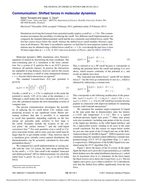
Figure 1 shows the basics of the LJ system. In the upper
figure the black curve gives the LJ pair potential u LJ (r) and the
black dashed curve the radial distribution function g(r), which
has its maximum close to u’s minimum. In the lower figure
the black (lower) curve shows the LJ pair force f LJ (r). The red
(upper) curve gives f SF (r) when a cutoff at 1.5σ is introduced;
note that the shifted force differs significantly from the true
force.
0021-9606/2011/134(8)/081102/4/$30.00 134, 081102-1
© 2011 American Institute of Physics
Downloaded 28 Feb 2011 to 130.226.173.81. Redistribution subject to AIP license or copyright; see http://jcp.aip.org/about/rights_and_permissions

081102-2 S. Toxvaerd and J. C. Dyre J. Chem. Phys. 134, 081102 (2011)
3
3
u(r) and g(r)
2.5
2
1.5
1
0.5
0
Radial distribution g(r)
2.5
2
1.5
1
0.8
0.7
0.6
1.4 1.5 1.6 1.7
–0.5
0.5
Force
–1
3
2
1
0
–1
–2
1 1.2 1.4 1.6 1.8 2
Radial distance r
FIG. 1. (a) The Lennard-Jones potential (black full curve) and the radial
distribution function g(r) (black dashed curve) for a system at ρ = 0.85
and T =1.00 in dimensionless units. (b) The radial force f LJ (r) =−u ′ LJ (r)
(black). At r = 1.5σ the force is 30 times larger than at r = 2.5σ .Also
shown is the shifted force for a cutoff at 1.5σ (red, upper curve).
Figure 2 shows the true pair-distribution function (black)
and the simulated g(r) forthreer c = 1.5σ cutoffs: SF (red,
barely visible), SP (green, slightly lower at r = 1.5σ ), and
a smoothed SP cutoff ensuring the force and its first derivative
go continuously to zero at the cutoff 12 [dashed (green)
curve]. The curves deviate little, except near the cutoff where
the smallest errors are found for a SF cutoff (inset).
In order to systematically compare the SP and SF cutoffs
we studied the LJ liquid for a range of cutoffs. Figure 3
quantifies the difference between the computed g(r) and
the true radial distribution function, g 0 (r), by evaluating
∫ 4.5σ
0
|g(r) − g 0 (r)|dr. SF is the red (lower) curve, SP is
the green (upper) curve. SF works better than SP for all
values of r c above the Weeks–Chandler–Andersen (WCA)
cutoff at the potential energy minimum 6 where SF = SP
(r c = 2 1/6 σ = 1.12σ ). Smoothing a SP cutoff has only a
marginal effect compared to not smoothing it (results not
shown). Applying first-order perturbation theory with the g(r)
obtained in a simulation with SF cutoff at r c = 1.5σ leads to
a pressure that deviates only 1% from the correct value.
Figure 4 studies energy drift in long NVE simulations
for r c = 1.5σ . The SF cutoff (red, horizontal) exhibits no energy
drift, whereas SP (green, diverging) does. Figure 4 also
gives results when the force of a SP cutoff is smoothed 12
(green dashed, horizontal curve). This leads to much better
energy conservation, 1 but the energy fluctuations are some-
0
1 1.2 1.4 1.6 1.8 2 2.2 2.4
Distance r
FIG. 2. Radial distribution function g(r) for the “true” LJ system (black) and
two cutoffs at r c = 1.5σ . The red (barely visible) curve gives results for a SF
cutoff, the green curve (slightly lower at r = 1.5) for a SP cutoff. The dashed
(green) curve gives results for a SP cutoff with smoothing of the force and
its derivative at the cutoff (Ref. 12); this, however, does not improve the SP
results.
what larger than for a SF cutoff. The simulations indicate
the existence of a hidden invariance in the central-difference
algorithm for a continuous force function, deriving from a
“shadow Hamiltonian.” 13
Not only static quantities, but also the dynamics are affected
little by replacing a 2.5σ SP cutoff with a 1.5σ SF
cutoff. This is demonstrated in Fig. 5, which shows simulations
of the incoherent intermediate scattering function of
the supercooled KABLJ liquid. 11 For reference a WCA cutoff
simulation is included (blue dashed curve, fastest relaxation),
which was recently shown to be inaccurate despite the
fact that the WCA radial distribution function is reasonably
good for this system. 14 A SP cutoff at r c = 1.5σ AA gives too
slow dynamics (purple dotted curve). Within the numerical
uncertainties incoherent scattering functions are identical for
Integral of abs(g(r)-g0(r))
0.1
0.08
0.06
0.04
0.02
0
u(min) f(min) g(min)
1.2 1.4 1.6 1.8 2 2.2 2.4
FIG. 3. Integrated numerical difference ∫ 4.5σ
0 |g(r) − g 0 (r)|dr of the true radial
distribution function, g 0 (r), and g(r) for various cutoff distances r c .The
red (lower) curve gives results for the SF cutoff, the green (upper) for the SP
cutoff. Smoothing a SP cutoff (Ref. 12) does not improve its accuracy (data
not shown).
r(c)
Downloaded 28 Feb 2011 to 130.226.173.81. Redistribution subject to AIP license or copyright; see http://jcp.aip.org/about/rights_and_permissions

081102-3 Shifted forces in molecular dynamics J. Chem. Phys. 134, 081102 (2011)
40
E(t)-E(0)
4
3
2
0.20
0.15
0.10
0.05
0
Force
30
20
10
0
1
-0.05
0 2E5 4E5 6E5 8E5
-10
-20
0
-30
0 2E7 4E7 6E7 8E7 10E7
Time t
FIG. 4. Energy drift as a function of time for long simulations (10 8 time
steps of length 0.005) with a cutoff at 1.5σ . The red (horizontal) curve gives
results for the SF cutoff, the green (diverging) for the SP cutoff, and the green
dashed (horizontal) curve for a smoothed SP cutoff. Smoothing a SP cutoff
stabilizes the algorithm, but the fluctuations are still somewhat larger than for
a SF cutoff. The inset shows the initial part of the simulation.
the “true” system, a SP cutoff at r c = 2.5σ AA , and a SF cutoff
at r c = 1.5σ AA . Similar results were found for the singlecomponent
LJ liquid’s dynamics. We conclude that a SF cutoff
at r c = 1.5σ generally works well for both statics and dynamics
of LJ systems.
Why does a cutoff, for which the forces are modified
at all distances (SF), work better than when the forces are
correct below the cutoff (SP)? A SF cutoff modifies the pair
force by adding a constant force for all distances below r c ;
at the same time SF ensures that the pair force goes continuously
to zero at r = r c . Apparently, ensuring continuity
of the force—and thereby that u ′′ (r) does not spike artificially
at the cutoff—is more important than maintaining
the correct pair force below the cutoff. How large is the
-40
0 100 200 300 400 500 600 700 800 900 1000
(a)
Time steps
Force
10
8
6
4
2
0
–2
–4
340 360 380 400 420 440
(b)
Time steps
FIG. 6. (a) The x component of the force on a typical particle during 1000
time steps. The black curve gives the true force, the red curve (barely visible
on top of the black curve) the force for a SF cutoff at 1.5σ . The blue curve
(fluctuating around zero) gives the sum of the x coordinates of the constant
“shift” terms of Eq. (3). (b) Details after 340 steps. The green (upper) curve
gives the SP force (r c = 1.5σ ). Only true and SF forces are smooth functions
of time.
F(q = 7.25,t)
1
0.9
0.8
0.7
0.6
0.5
0.4
0.3
0.2
0.1
0
0.01 0.1 1 10 100 1000 10000 100000
time
FIG. 5. The AA particle incoherent intermediate scattering function for the
KABLJ liquid in the highly viscous regime (T = 0.45, ρ = 1.2, q = 7.25).
In order from the left the figure shows results for: a WCA cutoff (blue dashed
curve), a SP cutoff at 2.5σ AA (green dashed curve), a SF cutoff at 1.5σ AA (red
full curve), the “true” system (black full curve), and a SP cutoff at 1.5σ AA
(purple dotted curve). Smoothing a SP cutoff (Ref. 12) does not improve its
accuracy (data not shown).
change induced by the added constant force of the SF cutoff?
Figure 6 shows the x component of the force on a typical
particle as a function of time (r c = 1.5σ ). The black curve
gives the true force, the red, barely visible curve the SF force,
and the blue, fluctuating curve the SF correction term. Although
the true and SF individual pair forces differ significantly
(Fig. 1), the difference between true and SF total
forces is small and stochastic (∼3%). This reflects an almost
cancellation of the correction terms deriving from the fact
that the nearest neighbors are more or less uniformly spread
around the particle in question. It was recently discussed why
adding a linear term (∝ r) to a pair potential hardly affects
dynamics 15 and statistical mechanics: 16 For a given particle’s
interactions with its neighbors the linear terms sum to almost
a constant because, if the particle is moved, some nearestneighbor
distances increase and others decrease, and their
sum is almost unaffected.
Figure 6(b) shows details of Fig. 6(a); we here added the
SP force for the same cutoff (green, upper curve). Both SP
and correction terms are discontinuous; they jump whenever
Downloaded 28 Feb 2011 to 130.226.173.81. Redistribution subject to AIP license or copyright; see http://jcp.aip.org/about/rights_and_permissions

081102-4 S. Toxvaerd and J. C. Dyre J. Chem. Phys. 134, 081102 (2011)
a particle pair distance passes the cutoff. Altogether, Fig. 6
shows that not only does the sum of the constant forces on
a given particle from its neighbors cancel to a high degree,
so do the interactions with particles beyond the cutoff. The
result is that the particle distribution is affected little by the
long-range attractive forces, a fact that lies behind the success
6, 17, 18
of perturbation theory.
In summary, when a SF cutoff is used instead of the
standard SP cutoff, errors are significantly reduced. Our
simulations suggest that a SF cutoff at 1.5σ maybeused
whenever the standard SP cutoff at 2.5σ gives reliable
results; this applies even though the pair force at r = 1.5σ
is 30 times larger than at r = 2.5σ . A cutoff at 1.5σ is
large enough to ensure that all interactions within the first
coordination shell are taken into account (Fig. 2). Use of a
1.5σ SF cutoff instead of a SP cutoff at 2.5σ leads potentially
to a factor of (2.5/1.5) 3 = 4.7 shorter simulation time for LJ
systems.
The center for viscous liquid dynamics “Glass and Time”
is sponsored by the Danish National Research Foundation
(DNRF).
1 M. P. Allen and D. J. Tildesley, Computer Simulation of Liquids (Oxford
Science Publications, Oxford, 1987); D. Frenkel and B. Smit, Understanding
Molecular Simulation (Academic, New York, 2002).
2 B. Smit, J. Chem. Phys. 96, 8639 (1992).
3 P. Grosfils and J. F. Lutsko, J. Chem. Phys. 130, 054703 (2009).
4 C. Valeriani, Z. J. Wang, and D. Frenkel, Mol. Simul. 33, 1023 (2007).
5 A. Ahmed and R. J. Sadus, J. Chem. Phys. 133, 124515 (2010).
6 J. D. Weeks, D. Chandler, and H. C. Andersen, J. Chem. Phys. 54, 5237
(1971); J. H. R. Clarke, W. Smith, and L. V. Woodcock, ibid. 84, 2290
(1986); J. D. Weeks, K. Vollmayr, and K. Katsov, Physica A 244, 461
(1997); F. Cuadros, A. Mulero, and C. A. Faundez, Mol. Phys. 98, 899
(2000).
7 S. D. Stoddard and J. Ford, Phys.Rev.A8, 1504 (1973); J. J. Nicolas, K.
E. Gubbins, W. B. Street, and D. J. Tildesley, Mol. Phys. 37, 1429 (1979);
J. G. Powles, W. A. B. Evans, and N. Quirke, ibid. 46, 1347 (1982).
8 D. Wolf, P. Keblinski, S. R. Phillpot, and J. Eggebrecht, J. Chem. Phys.
110, 8254 (1999); D. Zahn, B. Schilling, and S. M. Kast, J. Phys. Chem.
B 106, 10725 (2002); C. J. Fennell and J. D. Gezelter, J. Chem. Phys. 124,
234104 (2006).
9 For MD details see S. Toxvaerd, Mol. Phys. 72, 159 (1991). The unit length,
energy, and time used are, respectively, σ , ɛ, andσ √ m/ɛ.
10 L. Verlet, Phys. Rev. 159, 98 (1967).
11 W. Kob and H. C. Andersen, Phys. Rev. Lett. 73, 1376 (1994).
12 The radial force f SP (r) was smoothed in the interval r c ± δ by replacing
it with the function f (r) = f (r c − δ)h(x) with h(x) = 1 + cx
− (3 + 2c)x 2 + (2 + c)x 3 , where x = (r − r c + δ)/2δ and c = 2δu ′′
(r c − δ)/u ′ (r c − δ). This ensures that f SP and f SP ′ go smoothly to zero in
the cut interval. In the simulations δ = 0.025 (other values lead to similar
conclusions).
13 S. Toxvaerd, Phys.Rev.E50, 2271 (1994).
14 L. Berthier and G. Tarjus, Phys. Rev. Lett. 103, 170601 (2009); U.
R. Pedersen, T. B. Schrøder, and J. C. Dyre, ibid. 105, 157801
(2010); Y. S. Elmatad, D. Chandler, and J. P. Garrahan, J. Phys. Chem.
B 114, 17113 (2010).
15 N. P. Bailey, U. R. Pedersen, N. Gnan, T. B. Schrøder, and J. C. Dyre,
J. Chem. Phys. 129, 184508 (2008); T. B. Schrøder, N. P. Bailey, U. R.
Pedersen, N. Gnan, and J. C. Dyre, ibid. 131, 234503 (2009).
16 N. Gnan, T. B. Schrøder, U. R. Pedersen, N. P. Bailey, and J. C. Dyre, J.
Chem. Phys. 131, 234504 (2009).
17 J. A. Barker and D. Henderson, J. Chem. Phys. 47, 4714 (1967).
18 S. Toxvaerd, J. Chem. Phys. 55, 3116 (1971).
Downloaded 28 Feb 2011 to 130.226.173.81. Redistribution subject to AIP license or copyright; see http://jcp.aip.org/about/rights_and_permissions