A Benthic Terrain Classification Scheme for American Samoa

A Benthic Terrain Classification Scheme for American Samoa
Accepted for publication in Marine Geodesy, 2006
EMILY R. LUNDBLAD 1
DAWN J. WRIGHT
Department of Geosciences
Oregon State University
Corvallis, Oregon, USA
1 Now at Joint Institute for Marine and Atmospheric Research
University of Hawaii – Manoa
Contractor to NOAA Pacific Islands Fisheries Science Center
Honolulu, Hawaii, USA
JOYCE MILLER
Joint Institute for Marine and Atmospheric Research
University of Hawaii – Manoa
Contractor to NOAA Pacific Islands Fisheries Science Center
Honolulu, Hawaii, USA
EMILY M. LARKIN 2
RONALD RINEHART
Department of Geosciences
Oregon State University
Corvallis, Oregon, USA
2 Now at NOAA National Ocean Service
Silver Spring, Maryland, USA
DAVID F. NAAR
BRIAN T. DONAHUE
University of South Florida
St. Petersburg, Florida, USA
S. MILES ANDERSON
Analytical Laboratories of Hawaii, LLC
Honolulu, Hawaii, USA
TIM BATTISTA
NOAA National Centers for Coastal Ocean Science
Center for Coastal Monitoring and Assessment
Biogeography Program
Silver Spring, Maryland, USA
1

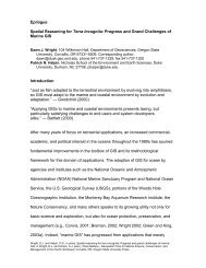
Abstract
Coral reef ecosystems, the most varied on earth, continually face destruction from
anthropogenic and natural threats. The U.S. Coral Reef Task Force seeks to characterize
and map priority coral reef ecosystems in the U.S./Trust Territories by 2009. Building
upon NOAA Biogeography shallow-water classifications based on Ikonos imagery,
presented here are new methods, based on acoustic data, for classifying benthic terrain
below 30m, around Tutuila, American Samoa. The results is a new classification scheme
for American Samoa that extends and improves the NOAA Biogeography scheme,
which, although developed for Pacific island nations and territories, is only applicable to
a maximum depth of 30 m, due to the limitations of satellite imagery. The scheme may be
suitable for developing habitat maps pinpointing high biodiversity around coral reefs
throughout the western Pacific.
2

Introduction
The high productivity of coral reef ecosystems demands a quantifiable analysis of
the complexity and diversity present there. Many people depend on the resources and
services that coral reef ecosystems provide, and the direct connection with adjacent
coastal ecosystems is important to increasing coastal populations (Culliton 1998).
Natural and anthropogenic processes threaten natural and cultural resources in these areas
in the form of storms, global warming, sea water level rise, disease, over-fishing, ship
grounding, sediment runoff, trade in coral and live reef species, marine debris, invasive
species, security training activities, offshore oil and gas exploration, and coral bleaching
(Miller and Crosby 1998; Evans et al. 2002). Although corals can recover from natural
disasters, their ecosystems may not bounce back in the face of destructive anthropogenic
threats (Miller and Crosby 1998; Weier 2001; Green et al. 1999).
The U.S. Coral Reef Task Force (CRTF) was established by NOAA in June 1998
as an overseer of coral reef protection. The CRTF Mapping and Information Working
Group has a goal to characterize and map all priority shallow water (30m) coral reef systems in the U.S. and Trust Territories by 2009
(Evans et al. 2002). Until 2001, U.S. coral reefs were not mapped at a resolution useful
enough for assessing and managing resources (i.e., multibeam bathymetry at 5-m
horizontal resolution or lower and extensive underwater video and photography along
transects). The work described here is a first step in meeting that objective for coral reef
systems around the island of Tutuila, American Samoa.
As growing populations flock to coastal homes, residents, resource managers,
researchers, scientists and other professionals alike are becoming more aware of the
3

importance of marine environments and their resources. To protect such environments
there is a need for documenting baseline information about them on an ecosystem level,
for long-term monitoring, and for estimating the geographic extent of critical habitats.
With this in mind, the National Oceanic and Atmospheric Administration’s (NOAA)
Biogeography Program turned to the use of satellite imagery to delineate potential
benthic habitats within coastal regions down to about 30 m (e.g., Monaco et al. 2005)
using a habitat classification scheme that is coral centric. By using heads-up digitizing to
analyze Ikonos imagery, airborne color aerial photography, and airborne hyperspectral
imagery, researchers have successfully classified habitats in much of the shallow water
regions around the coastal U.S. and Territories (i.e. Puerto Rico and the U.S. Virgin
Islands, Northwest Hawaiian Islands, Monterey Bay, American Samoa, the
Commonwealth of the Northern Mariana Islands, Guam) (Buja et al. 2002; Coyne et al.
2001, 2002a, 2002b, NCCOS 2005).
Scientists and researchers are extending their understanding to regions deeper
than 30 m in order to protect and monitor coral reef ecosystems, some of the most varied
on earth. To locate and study resources associated with particular terrains, it is necessary
to map benthic terrain at a fine-scale. New data collection and mapping techniques are
required to extend the shallow water classifications for potential habitats in deeper water,
at this fine-scale. The methods and results presented here explain a way to classify
benthic terrains in 30 to 150 m depths with a 1 to 2 m resolution. These terrains provide
information, based on an integration of marine data into a geographic information system
(GIS), which scientists may use to identify areas of high biodiversity and species’
potential habitats. Use and furtherance of the GIS and the resulting benthic terrain
4

classification may lead to more efficient management of marine protected areas, simpler
decision making with the use of more detailed, extensive, and accurate science,
advancements in marine and coastal research, and improvements on geo-referenced
marine mapping (e.g., Wright and Bartlett 2000; Valavanis 2002). In this case, layers
(i.e. multibeam bathymetry, slope, bathymetric position index (at multiple scales), and
rugosity) were combined in a GIS and assessed with unique algorithms to produce
classification maps.
A significant ongoing goal in seafloor exploration is to define a common
classification scheme that all characterization studies can use effectively and efficiently.
The development of a common classification scheme would make sharing results and
data easier. However, in this effort there is an understanding among researchers,
scientists, and managers that the use of a single, common classification scheme
applicable to all environments is not a reality yet. The seafloor mapping community is
striving for such a scheme at regional and local levels (e.g. MMUG 2003, Allee et al.
2000). The contribution of this paper is that it presents such a scheme specifically for
American Samoa, at depths of 30-150 m. This extends and improves the NOAA
Biogeography scheme, which, although developed for Pacific island nations and
territories, is only applicable to a maximum depth of 30 m, due to the limitations of
satellite imagery.
Review of Seafloor Classification Approaches: Multibeam and Visual Data
Most benthic terrain classification studies have relied primarily on analysis and
interpretation of multibeam bathymetry. They also had access to some kind of visually-
5

observed survey data (e.g., transect video, still photos, grab samples, etc.) to make
qualitative and/or quantitative inferences. Multibeam backscatter (i.e., the intensity of the
acoustic returns) has been used as well but is a separate issue, not discussed here, due to
the greater complexities in processing acoustic strength versus travel time, and of
interpreting seafloor sediment types and inhomogeneities in subbottom layers (as
explained in Zhou and Chen 2005).
Greene et al. (1999) developed a successful classification scheme for fish habitats
offshore of Central California. It was recently updated in Greene et al. 2005 and describes
broad classes such as megahabitats (based on depth and general physiographic
boundaries), meso/macrohabitats (based on scale), seafloor slope, seafloor complexity,
and geologic units. The scheme continues with more detailed habitat characteristics
interpreted from video, still photos or direct observation via SCUBA. They are
macro/microhabitats (based on observed small-scale seafloor features), seafloor slope
(estimated from in situ surveys), and seafloor complexity (estimated rugosity).
Weiss (2001) made a unique classification scheme for understanding watershed
metrics by using a topographic position and landform analysis. To form a topographic
position index (TPI), he used algorithms that perform an analysis on each grid cell in an
elevation model. Each grid cell is assigned a TPI value that indicates its position (higher
than, lower than, or the same elevation) in the overall landscape. By combining TPI with
slope position, Weiss (2001) found methods to apply a landform classification scheme to
watersheds around Mt. Hood, Oregon, USA and the west slope of the Oregon Cascades.
The scheme includes ten landform classes: canyons, deeply incised streams; midslope
drainages, shallow valleys; upland drainages, headwaters; U-shape valleys; plains; open
6

slopes; upper slopes, mesas; local ridges/hills in valleys, midslope ridges, small hills in
plains; mountain tops, high ridges. Weiss (2001) considered two scales of landforms in
order to incorporate structures found within broad landscapes. His techniques are well
suited to benthic classifications that serve as a predictor for habitat suitability and
biodiversity (Guisan et al. 1999).
Iampietro and Kvitek (2002) derived descriptive grids from multibeam
bathymetry to quantify seafloor habitats for the nearshore environment of the entire
Monterey peninsula in central California, USA with GIS. They followed Weiss’s (2001)
methods to develop TPI grids that, at a fine-scale, can describe micro- and macro-scale
habitats while, at a broad-scale, can describe meso- and mega-scale habitats. Another
derivative of bathymetry that they applied was rugosity. Rugosity is a measure of
roughness or bumpiness (classified as high, medium, and low) that is quantified with a
ratio of surface area to planar area.
Coops et al. (1998) further developed and tested procedures to predict topographic
position from digital elevation models for species mapping. In this study topographic
position is a “loosely defined variable” that attempts to describe topography with spatial
relationships. Quantitative assessments of such terrains are rarely reported. Topographic
position can help researchers understand how patterns, processes and species are spatially
related. While qualitative analyses can describe processes on slopes at different scales, a
quantitative assessment determines primary units within the context of a process.
Depending on the scale of the landscape in interest, more or fewer divisions of
topographic position may be quantified. This overview describes a landscape
classification scheme by Speight (1990). Speight (1990) defined morphology types with
7

eleven different classes: crests, depressions (open and closed), flats, slopes (upper, mid,
lower and simple), ridges, and hillocks. The topographic position analysis in this study
incorporates local relief, elevation percentile, plan and profile curvature, slope, and
variance threshold. After defining crests, depressions, flats and slopes, the study goes
further to define the more detailed classes. Unfortunately, the study does not attempt to
subdivide the depressions into open and closed though the classification scheme
recognizes the need for the distinction. Also, because of their fine scale complexity,
hillocks and ridges were not quantified (Coops et al. 1998).
Some historical studies have taken approaches to relate topographic features with
populations of particular species. Schmal et al. (2003) used multibeam bathymetric maps
to guide submersibles that allowed the researchers to identify detailed biotopes and
species within geomorphic zones (e.g. coral species zones within midshelf banks (< 36 m
depth) or within banks (< 50 m depth) or on the soft bottom). The bathymetry served as
an effective base layer in a GIS to use for their investigation. Another study that
effectively related species to their habitat locations used side scan sonar mosaics to find
the relationship between population abundance and the benthoscape (undersea
landscapes; Zajac et al. 2003). With the use of backscatter imagery, they classified large
scale benthoscapes such as muddy sands, fine sands and muds, boulder, cobble and
outcrop, sand wave fields, and mixed. They paid close attention to transitions between
benthoscapes where infaunal populations were readily identified at a finer scale.
The approach taken in the current study takes into consideration the many
applications of many types of data that are used for benthic habitat mapping (e.g. Hall et
al. 1999). Most often there is a need for a baseline of information. Usually, the baseline,
8

or framework, used for a habitat study is a basic data set that describes the surficial
characteristics of the seafloor in some useful fashion (Dartnell and Gardner, in press).
Then, based on what the seafloor looks like, a biologist, geologist, ecologist,
geophysicist, or other interested party will supplement that framework with specific data
sets. A biologist may add a layer of information about amount of relief or the thickness
of sediments. A geologist may add data revealing sediment size or rock type. Depending
on the interest of the research, different layers of information are needed. Therefore, a
method has been developed here that results in separate data sets that may be combined at
different scales and in different combinations to serve as a baseline of information for
researchers, scientists and managers. But as explained in the next section we combine this
with the satellite based approach NOAA Biogeography, considering and extending their
classifications into a new classification scheme for Pacific island deepwater habitats.
Existing NOAA Biogeography Approach: Satellite Imagery
NOAA’s Biogeography Program developed a classification scheme for benthic
habitats throughout the Pacific Islands (Coyne et al. 2002b), based on high-resolution
Ikonos satellite imagery, in order to meet the needs of resource managers and scientists.
This extends the approaches described in the previous section because with the synoptic
coverage of satellite imagery, it allows greater areas of the seafloor to be classified. The
drawback here, of course, is that it is only good to 30 m in clear waters. A hierarchical
classification was chosen to define and delineate habitats and was influenced by
management requests, the existing classification schemes, past knowledge of mapping
coral reefs, the minimum mapping unit, quantitative data, and limitations of the imagery
9

(Coyne et al. 2002b). Their hierarchical scheme uses two categories of classes (zones and
habitats) thereby allowing the user to expand and collapse the scheme. Zones describe a
benthic community’s location. Habitats, which occur within zones, are based on
geomorphologic structure and biological cover type. The structure and cover component
are then further divided into major and detailed levels resulting in a GIS polygon habitat
map product with each polygon populated with one zone and four habitat attributes. The
structural component of the maps is divided into four major and seventeen detailed
designations. The biological cover component is divided into nine major designations
with each subdivided into four density classes. Classes that were determined to be
undetectable from the imagery were not included in the scheme. This approach was first
developed by the Caribbean Fishery Management Council (Coyne et al. 2002b;
Christensen et al. 2003) and subsequently refined for use in Hawaii and the US Pacific
Territories.
In these maps, polygon boundaries are visually interpreted and manually
delineated on computer screen based of the color, texture and relative location of the
feature in the remotely sensed imagery. Extensive field observations are conducted to
determine habitat types in areas where uncertainty existed in the visual interpretation of
the imagery, where gradients exist through habitat types or where habitat diversity is
highly heterogeneous.
Field surveys were also conducted to acquire ground truth needed to establish a
statistically robust assessment of the thematic accuracy of these products (Congalton
1991; Rosenfield et al. 1982; Cohen 1960; Ma and Redmond 1995; Hudson and Ramm
1987). This statistical treatment generates over all accuracy, Kappa and Tau statistics as
10

well as user and producer accuracy of the thematic content of the map products at both
the major and detailed level of the classification scheme. Accuracy of the zone attribute
was not tested. Ikonos satellite imagery was used to generate all of these map products
for the coral reefs of American Samoa. The overall thematic accuracy was greater the
85% (Kappa and Tau >0.85) at the major level of the classification scheme and greater
then 75% (Kappa and Tau >0.75) for the detailed level of the classification scheme, but
again, only for a maximum depth of 30 m.
The classification scheme introduced in this paper bridges the multibeam
approaches of the previous section with the satellite-based approach of NOAA
Biogeography. Using those earlier approaches we effectively take the NOAA scheme into
deeper water. A primary objective of the current study was to extend this existing
classification below 30 m, the reach of what is viewable and classifiable in Ikonos
imagery.
Study Site and its Threats
American Samoa, a small, remote territory in the heart of the South Pacific, is the
only U.S. territory south of the equator and consists of about 197 km 2 of land cover. It
lies about 14 o south of the equator, about 4,700 km southwest of Honolulu, Hawaii
(Figure 1). It neighbors the independent nation of (western) Samoa as the eastern portion
of the Samoan archipelago. American Samoa’s five volcanic islands (Tutuila, Aunu’u,
Ofu, Olosega, and Ta’u) and two coral atolls (Rose and Swains) are surrounded by true
tropical reefs, which are extremely rare in U.S. waters.
11

Figure 1 Location Map of American Samoa. A U.S. Territory that is home to priority
coral reefs that are part of the National Action Plan to Conserve Coral Reefs. American
Samoa is part of the Samoan archipelago and is comprised of 5 volcanic islands and 2
coral atolls.
The coral reef ecosystems around American Samoa are being threatened by natural
and adverse anthropogenic patterns and processes (Evans et al. 2002). For example, coral
bleaching events related to sea temperature rise have increased in the region, including a
particularly destructive event in 1994 (FBNMS 2004). An infestation of crown-of-thorns
starfish killed vast amounts of coral in the late 1970s owing to their habits of eating live
coral (Craig 2002). In addition, coral around the South Pacific islands are threatened
annually by tropical cyclones. American Samoa suffered from the effects of hurricane
Ofa in 1990, hurricane Val in 1991, and most recently hurricane Heta in January 2004
(Craig 2002; FBNMS 2004; FEMA 2004). Anthropogenic threats such as gill netting,
12

spear fishing, poison and dynamite fishing, non-point pollution and cumulative impacts
challenge and stunt coral reef recovery from natural disasters (ASG: DOC 2004).
Deep Water (30 m – 200 m) Data Collection for This Study
Extensive data have been collected in American Samoa since 2001 including
multibeam bathymetry, towed diver videos, accuracy assessment photography, field
notes, and information from a rebreather dive (Wright 2002; Wright et al. 2002).
Multibeam mapping systems allow surveyors to collect bathymetry by ensonifying
massive areas of the seafloor with high accuracy (e.g., Blondel and Murton 1997; Mayer
et al. 2000). Scores of acoustic beams form a swath that fans out up to several times the
water depth. Multibeam mapping systems are set up on research vessels that navigate
across the study area making real-time adjustments for sound velocity, heave, roll, pitch,
and speed (3-12 knots) (e.g., Blondel and Murton 1997). Most modern multibeam
mapping systems also collect backscatter data which are often useful for classifying
seafloor bottom characteristics (e.g., sediments versus lava flows).
The first scientific surveys of depths beyond 30 m in coral reef ecosystems
around American Samoa collected bathymetric data from 3 to 160 m depth in 2001 and
2002 with the University of South Florida’s Kongsberg Simrad EM3000, 300 kHz,
multibeam mapping system (Wright et al. 2002; Wright 2002). The 2001 survey
collected bathymetry and backscatter for Fagatele Bay National Marine Sanctuary
(FBNMS), part of the National Park, Pago Pago Harbor, the western portion of Taema
Bank, and Faga’itua Bay (Figure 2). Sites surveyed in November 2002 are eastern
Taema Bank, Coconut Point, Fagatele Bay, and Vatia Bay (Figure 2).
13

Figure 2. Location of high-resolution multibeam bathymetry surveys around Tutuila,
American Samoa (1-m horizontal spatial resolution and +1-m vertical accuracy for all
areas except for the National Park where data were collected at 2-m resolution with a
vertical accuracy of ~+5 m). Projection: Geographic, WGS84. Bathymetry was
collected in April and May of 2001 and November of 2002 with the Kongsberg Simrad
EM3000 (http://dusk.geo.orst.edu/djl/samoa ).
The NOAA Coral Reef Ecosystem Division (CRED), part of the Pacific Island
Fisheries Science Center (PIFSC), conducted surveys in February/March 2002 and
February/March 2004. CRED towed diver video (0 – 25 m), deeper (20 – 100 m) towed
photographic and video data, and single beam/bottom classification data resulting from
the 2002 surveys were used for this analysis. Extensive multibeam (bathymetry and
backscatter) and video data were also collected in early 2004, but it was not possible to
incorporate these data here. These multibeam bathymetric data are now available online
at http://www.pifsc.noaa.gov/cred/hmapping.
14

Data Analysis and Processing
Bathymetry
300 kHz multibeam bathymetry data from the 2001 and November 2002 surveys
were used for analysis, after post-processing, as a 3-column XYZ ASCII file with
positive depth values based on a mean low low water datum at full resolution of the
Kongsberg Simrad EM3000 system. For Fagatele Bay, Coconut Point and Taema
(Eastern), the XYZ bathymetry was gridded at 1m spacing in MB-System (Caress et al.
1996). MB-System outputs grids in the format of Generic Mapping Tools (GMT) for a
UNIX environment. GMT is a public suite of tools used to manipulate tabular, timeseries,
and gridded data sets, and to display these data in appropriate formats for data
analysis (Wessel and Smith 1991). Then the GMT grids were converted to a format
compatible with Arc/INFO® using a suite of tools called ArcGMT (Wright et al. 1998).
For Taema Bank (Western), the XYZ data were gridded with Fledermaus and exported as
an ArcView ASCII file, then converted to a grid with ArcToolbox. After importing the
grids into the Arc/INFO® raster grid format, algorithms were run in ArcGIS to
calculate derivatives.
Bathymetric Derivatives: Bathymetric Position Index, Slope
First, positive depth values were converted to negative. Slope, or the measure of
steepness first-order derivative, was simply derived using the ArcGIS spatial analyst
extension’s surface analysis. Output slope values (raster grids) are derived for each cell
as the maximum rate of change from the cell to its neighbor.
15

Bathymetric Position Index (BPI) is a second-order derivative (as it is derived
from the first derivative, slope) of bathymetry as modified from topographic position
index as defined in Weiss (2001) and Iampietro and Kvitek (2002). BPI was derived as a
measure of where a georeferenced location, with a defined elevation, is relative to the
overall landscape. The derivation involves evaluating elevation differences between a
focal point and the mean elevation of the surrounding cells within a user defined
rectangle, annulus, or circle.
For example, where a user has an elevation grid that has 1 meter resolution,
he/she may choose to analyze the grid with an annulus. The annulus, having an inner
radius of 2 units and an outer radius of 4 units, would be used to spatially analyze each
grid cell in comparison to its neighboring cells that fall within that annulus (Figure 3).
Figure 3 Example of the variables used to derive bathymetric position index (BPI) from
bathymetry. The grid cells here (1 m resolution) represent bathymetry as negative values.
The annulus has an outer radius of 4 and an inner radius of 2. Therefore the BPI
scalefactor is 4 (outer radius multiplied by bathymetry resolution).
16

BPI was calculated in the ArcGIS raster calculator using the focal mean
calculation described above; the resulting grid values are converted to integers to
minimize the storage size of the grid and to simplify symbolization (Algorithm 1).
Algorithm 1 creates a BPI grid using bathymetry and user defined radii:
scalefactor = outer radius in map units multiplied by bathymetric data resolution
irad = inner radius of annulus in cells
orad = outer radius of annulus in cells
bathy = bathymetric grid
rad = radius (if using circle instead of annulus)
BPI = int((bathy – focalmean(bathy, annulus, irad, orad)) + 0.5)
OR
BPI = int((bathy – focalmean(bathy, circle, rad)) + 0.5)
The cells in the output grid are assigned values within a range of positive and
negative numbers (Figure 4). The 0.5 is added before the integer conversion and is meant
to force floating point values, regardless of the sign of the value, to round up if the value
has a decimal of greater than .5 and to round down if the value has a decimal of less than
.5. The variable is not necessary if a user chooses to allow the floating point values to be
rounded downward consistently for positive and negative values.
17

Figure 4 A description of the resulting bathymetric position index (BPI) values that are
derived from bathymetry. These are based on a topographic position index by Weiss
(2001). (Top) describes fine scale BPI values. (Bottom) describes broad scale BPI
values. (Courtesy of Weiss 2001)
A negative value represents a cell that is lower than its neighboring cells (valleys).
A positive value represents a cell that is higher than its neighboring cells (ridges). Larger
numbers represent benthic features that differ greatly from surrounding areas (such as
sharp peaks, pits or valleys). Flat areas or areas with a constant slope produce near-zero
values.
In this example, the cells with a value of 1 are higher than those with the value of
0, and the values of 2 are higher than the others (Figure 5). The diagonally linear pattern
of cells with the value of 1 starting from the top, left corner of the grid may represent a
crest in the benthoscape. Furthermore, the grid cells with values of 2 along that pattern
may be narrow crests on top of the larger crest. Also, notice that the other groups of BPI
values of 1 may represent small mounts within the benthoscape. The values of 0 are all
flat areas or constant slopes. Whether they are flats or slopes would be determined in
another algorithm that considers slope along with BPI. This derivation is discussed in the
development of classification scheme for American Samoa section. This example does
not include negative BPI values. If negative values were present in this grid sample, they
18

would represent patterns of depressions. The scalefactor of the resulting grid is 4, where
scalefactor is the resolution multiplied by the outer radius.
Figure 5 Example of the variables used to derive bathymetric position index (BPI) from
bathymetry. The grid cells represent a derived BPI grid. Negative values are lower than
their neighbors. Positive values are higher than their neighbors. Values of zero are flat
areas or areas with constant slope.
The results of BPI are scale dependent; different scales identify fine or broad
benthic features. To achieve the best BPI zone and structure classifications several large
and small-scale grids were created for each study site. The fine scale grids were created
with scalefactors of 10, 20, and 30, and the broad scale grids were created with
scalefactors of 50, 70, 125, and 250. BPI and BPI were used to classify
Fagatele Bay and Taema Bank. These scalefactors were chosen because, at these sites,
the small seascape features (distance between relatively small ridges) are, on average,
about 20 m across; the large seascape features (e.g. the distance across the deep channel
on the west end of Taema Bank and the length of the peninsula in Fagatele Bay) are
about 250 m across. This is based on close examination of the bathymetry prior to the
19

BPI calculation, especially in the Fledermaus 3-D visualization system. For Coconut
Point, features of interest were identified from about 10 m to 70 m across, so BPI
and BPI were used. See Tables 1 and 2 for the values used to derive BPI for each
study site.
Study Site
Resolution
(meters)
circle,
annulus, or
rectangle
Radius
Fagatele Bay 1 circle 20 20
Coconut Point 1 circle 10 10
Taema Bank 1 circle 20 20
2002 (Eastern)
Taema Bank
2001 (Western)
1 circle 20 20
Fine
Scalefactor
Table 1 Parameters used for calculating fine scale bathymetric position index grids
Study Site
Table 2 Parameters used for calculating broad scale bathymetric position index grids
Prior to the classification of the final zones and structures, BPI was standardized.
Conclusions about the structure of the overall seascape can be made with spatial analysis
by applying an algorithm that combines standardized BPI grids of different scales with
slope and bathymetry. In Arc/INFO® GRID, the final algorithms for classifying BPI
zones and structures are based on combined broad scale and fine scale standardized BPI
grids, slope, and depth.
Resolution
(meters)
circle,
annulus, or
rectangle
Irad Orad Broad
Scalefactor
Fagatele Bay 3 annulus 16 83 250
Coconut Point 1 circle 70 70
Taema Bank 3 annulus 16 83 250
2002 (Eastern)
Taema Bank
2001 (Western)
3 annulus 16 83 250
20

Rugosity Analysis
The rugosity analysis resulted in descriptive maps that help identify areas with
potentially high biodiversity. Rugosity describes topographic roughness with a surface
area to planar area ratio. Rugosity was derived with the ArcView® Surface Area from
Elevation Grids extension (Jenness 2003) using a 3x3 neighborhood analysis to calculate
surface area based on a 3D interpretation of cells’ elevations. Rugosity values near one
indicate flat, smooth locations; higher values indicate areas of high-relief. Rugosity
calculated using this technique is highly correlated with slope. The highest rugosity
values show a relationship with the high slope and lower rugosity with low slope.
Rugosity classifications extend the classes used by CRED for habitat complexity in their
2002 towed-diver surveys. The classes were assigned with the following standard
deviation divisions in ArcView® 3.3: Very High (>3 std. dev.), High (2–3 std. dev.),
Medium High (1–2 std. dev.), Medium (0–1 std. dev.), Medium Low (Mean), Low (-1–0
std. dev.). Rugosity can be associated with attributes recorded during dives and with
comments and attributes recorded in accuracy assessment surveys conducted in 2001
(Figure 6). From qualitative analysis, the derived rugosity grid and the towed-diver
surveys are not directly related. However, from this type of comparison, divers may
possibly standardize their observations among different divers in order to collect less
subjective information about the environment.
21

Figure 6 Rugosity derived in ArcView® 3.3 and towed-diver video transects symbolized
by habitat complexity observations. Transects overlaid on rugosity grid shows the
relationship between the two data sets.
Development of Classification Scheme for American Samoa
Since post-processing of the 2001 and 2002 data was completed during the initial
phase of this study, only these multibeam bathymetry data were used to classify the
seafloor on the basis of bathymetric position index (BPI) and rugosity. The methods
developed were based on the topographic position index algorithms of Guisan et al.
(1999), Weiss (2001) and Iampietro and Kvitek (2002) and the rugosity algorithm of
Jenness (2003) as applied in Iampietro and Kvitek (2002). Their application to American
Samoa bathymetry is the first extension of existing shallow water benthic classification to
depths beyond 30 m. (Figure 7).
22

Figure 7 The amount of overlap that exists between NOAA Biogeography habitat
classifications that were made using Ikonos imagery and the coverage of multibeam
bathymetry as of 2002.
Spatial analysis was used to derive, from the original bathymetry, indices of slope
and multiple scales of BPI (i.e., BPI zones and structures). The resulting derivative grids
were combined with a new algorithm to develop final products: BPI zones, BPI structures
and rugosity classification maps for the study sites. The maps introduce the first
deepwater benthic classification scheme for American Samoa that may also be extended
to other coral reef systems. The mapping steps for the classifications, including the
classification scheme, are summarized in the flowchart in Figure 8. The process
identifies four BPI zones and thirteen structure classes.
23

Figure 8 A Flowchart showing the data sets used to derive BPI zones and structures.
The algorithm that combines these data sets uses standard deviation units where 1
standard deviation is 100 grid value units; slope and depth values are defined by the user.
The algorithms for BPI zones and structures use different combinations of the grids. The
following is an example of how BPI zones were derived (Algorithm 2).
Algorithm 2 creates an output grid classified by BPI zones by combining the attributes of
BPI and slope:
B-BPI = broad scale BPI grid
out_zones = name of the output grid
slope = the slope grid derived from bathymetry
gentle = the user defined slope value indicating a gentle slope
if (B-BPI >= 100) out_zones = 1
else if (B-BPI -100 and B-BPI < 100 and slope -100 and B-BPI < 100 and slope > gentle) out_zones = 4
endif
24

The unique numbers assigned to classes in algorithm 2 are the following, as defined in
the classification scheme for BPI zones: (1) Crests, (2) Depressions, (3) Flats, and (4)
Slopes.
Structures were derived with a similar algorithm as that used for BPI zones,
however both scales of BPI were considered in order to pinpoint finer features. Also, the
variable of depth was added to identify different flat structures that may represent
different habitats. The decision tree below shows the path of decisions that the algorithm
uses to derive structure classes (Figure 9). The algorithm assigns a unique number to
each of the thirteen structures. The unique numbers assigned to classes are the following,
as defined in the classification scheme for structures: (1) Narrow depression, (2) Local
depression on flat, (3) Lateral midslope depression, (4) Depression on crest, (5) Broad
depression with an open bottom, (6) Broad flat, (7) Shelf, (8) Open slopes, (9) Local crest
in depression, (10) Local crest on flat, (11) Lateral midslope crest, (12) Narrow crest, and
(13) Steep slope.
25

Figure 9 A flowchart of the decisions made by the algorithms that derive zone and
structure classes from broad scale bathymetric position index (B-BPI), fine scale BPI (F-
BPI), slope and depth.
Specific values for slope and depth are sensitive to interpretation at specific study
sites. Each study site has a unique composition of depth and slope ranges. The methods
are best applied where slope and depth values are considered on the condition of
transition zone locations and the presence of two or more significant depth ranges within
the study site. In order to develop a uniform classification for all the American Samoa
study sites, common values that are suitable for sites around Tutuila were used in the
classification algorithms. Gentle slopes were defined 5° and steep slopes were defined as
70°. A depth of -22 m was used to define the difference between shelves and broad flats.
These slopes and depths were determined using 3D visualization in Interactive
Visualization System’s Fledermaus software.
26

Multiple schemes were reviewed to aid in the development of classifications for
the reefs of American Samoa (Coops et al. 1998; Dartnell and Gardner 2004; Greene et
al. 1999; Iampietro and Kvitek 2002; Schmal et al. 2003; Speight 1990; Zajac et al. 2003;
White et al. 2003; Greene et al. 2005). Weiss’s (2001) landform scheme is also valuable
as it classifies slope position and landform types as predictors of habitat suitability,
community composition, and species distribution. In this study, similar landform classes
are interpreted only to describe the seafloor and as a baseline for future habitat studies,
given the availability of future data on species counts and distributions. The terminology
used in the classification scheme (for zones) presented here is well-matched with the
NOAA/NOS Biogeography Program’s scheme for shallow water classifications (NWHI
2003). This biogeography scheme is being extended into deeper water by scientists at
CRED are working primarily with multibeam and underwater video data (Rooney and
Miller pers. comm. 2004) in 20-200m water depths. The NOAA/NOS classification
schemes, the Weiss (2001) landform scheme, and the Speight (1990) scheme, were
closely analyzed to develop agreeable terms for the BPI zones and structures that extend
below 30 m depth around American Samoa.
In this scheme, broad refers to seafloor characteristics defined by broad scale BPI
grids and fine refers to seafloor characteristics defined by fine scale BPI grids. BPI has
been described in more detail in the data analysis section.
Classification Scheme for BPI Zones
A surficial characteristic of the seafloor based on a BPI value range at a broad
scale and on slope values.
27

Figure 10 BPI Zones for Fagatele Bay National Marine Sanctuary.
1. Crests - High points in the terrain where there are positive bathymetric position
index values greater than one standard deviation from the mean in the positive
direction
2. Depressions - Low points in the terrain where there are negative bathymetric
position index values greater than one standard deviation from the mean in the
negative direction
3. Flats - Flat points in the terrain where there are near zero bathymetric position
index values that are within one standard deviation of the mean. Flats have a
slope that is 5 o . Slopes are otherwise called escarpments in the
NOAA/NOS classification scheme.
28

Classification Scheme for Structures
A surficial characteristic of the seafloor based on a BPI value range at a combined
fine scale and broad scale, on slope values and on depth.
Figure 11 Structures for Fagatele Bay National Marine Fisheries.
1. Narrow depression - A depression where both fine and broad features within
the terrain are lower than their surroundings
2. Local depression on flat - A fine scale depression within a broader flat terrain
3. Lateral midslope depression - fine scale depression that laterally incises a slope
4. Depression on crest - A fine scale depression within a crested terrain
5. Broad depression with an open bottom - A broad scale depression with a U-
shape where any nested, fine scale features are flat or have constant slope
29

6. Broad flat - A broad flat area where the terrain contains few, nested, fine scale
features
7. Shelf - A broad flat area where the terrain contains few, nested, fine scale
features. A shelf is shallower than 22 m depth. (This depth value was decided
on based on 3D visualization and the NOAA/NOS classification scheme
(NWHI 2003). The NOAA/NOS scheme defines a shelf as ending between 20
and 30 m depth.)
8. Open slopes - A constant slope where the slope values are between 5 o and 70 o
and there are few, nested, fine scale features within the broader terrain.
9. Local crest in depression - A fine scale crest within a broader depressed terrain
10. Local crest on flat - A fine scale crest within a broader flat terrain
11. Lateral midslope crest - A fine scale crest that laterally divides a slope. This
often looks like a ledge in the middle of a slope
12. Narrow crest - A crest where both fine and broad features within the terrain
are higher than their surroundings
13. Steep slope - An open slope with a slope value greater than 70 o
Discussion
The classification developed in this study is the first for deepwater environments
in American Samoa and should make a critical contribution to benthic habitat mapping in
the Pacific. It gives a unique picture of coral reef environments on two different scales.
The descriptive name of each class in the scheme provides users a way to recognize
patterns of terrain based on zones and structures. The classification uses general terms
that can apply to coral reef environments as seen by scientists with several different
interests (e.g. biological habitats, coral disturbance after natural disasters, algae growth,
and marine mammal distribution). By using general descriptions of the zones and
structures based on the analytical procedures described in this paper, researchers and
scientists may view coral reef environments with the focus of most specialties. The
30

classifications advantageously use several data sets to describe basic features of the coral
reef environment. The basic descriptions, using standard language among other
classifications schemes, allow the classifications to be used for qualitative analyses or for
quantitative analyses. The quantitative nature would be accomplished from raster
calculations to determine spatial statistics within and among the classes. One
disadvantage to the classification is that the scheme does not incorporate shape of
features. For instance, if a crest is linear it should be recognizable by sight as a linear
ridge. However, the classification scheme will not indicate the difference between a
group of crests that form a linear ridge and a group that forms a mound. The same
challenge exists for classifying patterns of depressions (i.e. channels vs. holes).
The classification does not provide a complete description of benthic habitats, but
adds to the resources that may be used in an integrated GIS. By using multibeam
bathymetry and derivative data sets to describe the structures of the seafloor, researchers
have a better idea of how to combine the data in a fashion that will answer important
scientific questions. While the resulting data sets (BPI zones, structures, and rugosity)
each provide a unique picture of the benthic environment, a combined analysis may
reveal more, important information. Researchers at CRED are using the data sets in an
integrated GIS in order to make products that may be used by working scientists and
managers. The integration of marine data in GIS provides a means for advancing marine
and coastal research, science and management, geo-referenced mapping, modeling and
decision making (e.g., Wright and Bartlett 2000; Valavanis 2002; Greene et al., 2005).
The integration of the unique data sets in a GIS will allow researchers and scientists to
query the data based on any combination of all of the available data sets. For example, a
31

habitat for a particular fish may be indicated by depths between 30 and 45 meters, where
many small crests and depressions are interlaced at a fine scale, having high rugosity. A
user can query all the data sets at one time within the integrated GIS in order to create a
new data set that includes only the habitats that meet those criteria. Also, a user may
merge data sets for adjacent areas to make a regional analysis, or a user may choose to
make a simple qualitative analysis of all the data sets in order to plan sampling locations
for in situ data collection.
The data analyzed in a GIS are validated when combined with in situ data sets.
Such groundtruthing (i.e. video collection, still photos, diver rugosity measurements) was
collected in the shallow waters (< 30 m) around Tutuila in February/March 2002 and
2004 and along the west coast of Saipan in the Commonwealth of the Northern Mariana
Islands in December 2004. Currently, scientists at CRED are analyzing the in situ data in
order to make a more informed accuracy assessment of the data sets derived in this study.
The method and classification scheme were tested with the bathymetry from the Saipan
anchorage area. Resulting BPI grids were made for zones and for structures using the
classification scheme discussed in this paper. The underwater videos were classified
using a scheme developed for optical validations data around coral reef ecosystems in
Pacific Island regions. The scheme does not match the one presented in this paper, but
the results are promising as they qualitatively present an immediate association between
the BPI structures and underwater video classifications. For example, where raised
features outlined by open slopes (e.g. shelves) are characterized in the BPI structures the
videos were classified as hard bottom (e.g. rock). Likewise, where broad flats are located
the videos reveal unconsolidated (e.g. sand) substrate. The open slopes and other
32

transitional areas (e.g. narrow crests and lateral midslope features) often correspond with
mixed substrates or rubble. This analysis is continuing to find relationships between BPI
zones/structures and percentages of living cover (e.g. Coralline Algae, Scleractinian
Coral, Macroalgae), scale of relief (i.e. 5 categories ranging from less than 0.5 m - > 3.0
m), and number/size of cavities noted in the frame (e.g. few small and many large
cavities, many small cavities). The analysis is evolving into a product that will validate
interpolations of coral cover and substrate type across the region; it will eventually
provide a prototype habitat map and methods that may be applied to other Pacific Island
regions.
Figure 12 BPI Structures overlaid with optical validation. This is a sample from the
Saipan anchorage data set that was surveyed by CRED in 2003 and 2004. The structures
were derived from a bathymetric grid (5-m pixel size), and the optical validation
represents interpretations of videos from a towed underwater video camera-sled. A
qualitative assessment validates a pattern of associations between substrates and BPI
structures.
33

Additionally, during CRED’s mission in early 2004, a complete backscatter data
set was collected and is, as of August 2005, available for download at
http://www.nmfs.hawaii.edu/cred/hmapping/hmap_data.php. The backscatter is an
enormous asset to determining potential benthic habitats. By incorporating it in the GIS,
patterns of the types and/or composition of substrate may be exposed within each zone,
structure and rugosity class. Our scheme will be further validated by recent Pisces V
submersible dives to Fagatele Bay and Taema Bank on Hawaii Undersea Research Lab
cruise KOK0510, along with the accompanying statistical validation, July 2005 (Wright
et al, in prep; http://dusk.geo.orst.edu/djl/samoa/ hurl ).
All of the analytical procedures used for the classifications in this study have been
encapsulated into a convenient GIS desktop tool called the Benthic Terrain Modeler
(BTM; Rinehart et al. 2004; http://www.csc.noaa.gov/products/btm). This ArcGIS 8.x/9.x
extension was jointly developed by researchers at Oregon State University and the
NOAA Coastal Services Center. It should allow the user to replicate the procedures on
the bathymetry used in this study (now permanently archived and publicly available at
http://dusk.geo.orst.edu/djl/samoa ), on CRED datasets, or on the user’s own dataset. The
BTM will allow users to apply the classification scheme used in this study for Tutuila on
their own coral reef bathymetry. The user may use the default classification scheme, as
described in this paper, or they may develop or insert other schemes in XML format
(Rinehart et al. 2004). The benthic mapping methods may potentially be applied to other
study sites around American Samoa and to coral reef ecosystems across the Pacific and in
the Caribbean. The application of the methods to extend shallow water classifications
will be fairly easy with the use of the BTM.
34

Conclusion
The study was a success in reaching its goals: (1) methods were developed for benthic
mapping and applied to 3 sites around American Samoa, (2) a new classification scheme
was developed introducing the concepts of BPI zones at a broad resolution (depressions,
slopes, flats, crests) and structures (finer features within zones) around the study sites and
supplemented by measures of rugosity, where complex features may be hosting high
biodiversity; and (3) visual survey information was used as initial validation for the
resulting classifications.
Bathymetry, BPI, slope, and rugosity were combined with spatial analysis to
develop methods for creating a classification for deep water (> 30 m) benthic zones and
rugosity around American Samoa. The methods were based on components of studies
that classified shallow water coral reef systems, terrestrial landforms, but also the
satellite-based (Ikonos) classification of NOAA Biogeography for Pacific islands. From
these shallow water classifications, only the zones, at a macro habitat level (Greene et al.
1999) were suitable for extension to deep water sites. The methods used for the deep
water benthic zone and rugosity classifications around American Samoa extend the
classifications for shallow waters around the territory.
As American Samoa is an archipelago of mostly submerged volcanoes, its
shoreline is flanked by fringing reefs that plunge into deep water. This dramatic
topography, combined with a tropical climate, creates a complex coral reef ecosystem
that supports thousands of species. BPI zones, structures and rugosity provide a
framework for planning scientific surveys that will give a better understanding of specieshabitat
relationships and possibly for establishing and monitoring marine protected areas.
35

Future studies include the work of NOAA CRED in interpreting additional extensive
towed video footage around Tutuila, as well as Saipan, to further validate our
classification scheme and assess its utility to other islands beyond Samoa, and the
analysis of Pisces V submersible dive videography just collected in July 2005 on Hawaii
Undersea Reserch Lab cruise KOK0510. As the results become available, they will
provide a tool for statistical analysis along video transects and for areas interpolated
between them. The statistical results may help to define a more automated process for
using bathymetric derivatives (e.g. BPI zones, structures, rugosity, texture) to create
habitat classifications.
The classifications resulting from the methods in this study, when combined with
associated marine life information, are tools for designing management programs for the
Fagatele Bay National Marine Sanctuary, the National Park of American Samoa, and
other marine reserves in the territory. They are a baseline of information for policy
makers and managers to establish a wider and more effective network of marine
protection throughout the Pacific contributing also to a national and global investigation
of the world’s marine and coastal environment.
36

Acknowledgements
This research was supported by NOAA Coastal Services Center (CSC) Special
Projects for the Pacific Islands Initiative, Grant #NA03NOS4730033 to D. Wright and
additional NOAA support to D. Naar. We acknowledge the logistical and financial
support from Marine Sanctuary Director, Nancy Daschbach, as well as the warm
hospitality provided by the local villages adjacent to Fagatele Bay and Vatia Bay. Others
instrumental in this project were Will White (formerly of Department of Marine and
Wildlife Resources), John Rooney (CRED), Peter Craig (National Park of American
Samoa (NPAS)), Allison Graves (formerly of NPAS), Curt Whitmire (NOAA Northwest
Fisheries Science Center), Anita Grunder (Oregon State University), Joshua Murphy and
Lori Cary-Kothera (CSC), Jeff Jenness (Jenness Enterprises), Pat Iampietro (California
State University, Monterey Bay), and Will Smith (Hawaii Institute of Marine Biology).
The comments of two anonymous reviewers significantly improved the manuscript.
37

References
American Samoa Government: Department of Commerce (ASG: DOC). 2004. American
Samoa Coastal Management Program. http://www.amsamoa.com/coastmgmt.htm
Blondel, P. and B. J. Murton. 1997. Handbook of Seafloor Sonar Imagery. Chichester,
U.K.: John Wiley & Sons.
Buja, K., M. Kendall, and C. Kruer. 2002. Mapping the benthic habitats of Puerto Rico
and Virgin Islands: A spatial framework for coastal zone management. In
Proceedings of the 22nd Annual ESRI User Conference. San Diego, CA, July 8-
12. http://gis.esri.com/library/userconf/proc02
Caress, D.W., S.E. Spitzak, and D.N. Chayes. 1996. Software for multibeam sonars.
Sea Technology. 37: 54-57.
Christensen, J.D, C.F.G. Jeffrey, C. Caldow, M.E. Monaco, M.S. Kendall, and R.S.
Appeldoorn. 2003. Quantifying habitat utilization patterns of reef fishes along a
cross-shelf gradient in southwestern Puerto Rico. Gulf and Caribbean Research.
14(2):1-15.
Cohen, J. 1960. A coefficient of Agreement for Nominal Scales. Educ. Psychol.
Measurement. 20(1): 37-46.
Congalton, R. 1991. A Review of Assessing the Accuracy of Classifications of Remotely
Sensed Data. Remote Sensing of Environment. 37: 35-46.
Coops, N., P. Ryan, A. Loughhead, B. Mackey, J. Gallant, I. Mullen, M. Austin. 1998.
Developing and Testing Procedures to Predict Topographic Position from Digital
Elevation Models (DEM) for Species Mapping (Phase 1). In CSIRO Forestry and
Forest Products: Client Report NO. 271.
Coyne, M.S., M.E. Monaco, M. Anderson, W. Smith, and P. Jokiel. 2001. Classification
Scheme for Benthic Habitats: Main Eight Hawaiian Islands. National Oceanic
and Atmospheric Administration: Silver Spring, MD. http://biogeo.nos.noaa.gov/
projects/mapping/pacific/main8/classification
Coyne, M.S., M.E. Monaco, M. Anderson, W. Smith, and P. Jokiel. 2002a. Classification
Scheme for Benthic Habitats: Northwest Hawaiian Islands. National Oceanic and
Atmospheric Administration: Silver Spring, MD. http://biogeo.nos.noaa.gov/
projects/mapping/pacific
Coyne, M.S., M.E. Monaco, M. Anderson, W. Smith, and P. Jokiel. 2002b. Classification
Scheme for Benthic Habitats: U.S. Pacific Territories. National Oceanic and
Atmospheric Administration: Silver Spring, MD. http://biogeo.nos.noaa.gov/
projects/mapping/pacific/territories
38

Culliton, T. J. 1998. Population: Distribution, Density and Growth. In NOAA’s State of
the Coast Report. http://state-of-coast.noaa.gov/bulletins/html/pop_01/pop.html
Craig, P. 2002. Natural History Guide to American Samoa. National Park of American
Samoa: Pago Pago, American Samoa.
Dartnell, P. and J.V. Gardner. 2004. Predicting Seafloor Facies from Multibeam
Bathymetry and Backscatter Data. In Photogrammetric Engineering and Remote
Sensing. 70(9): 1081.
Diaz, J. V. M. 2000. Analysis of Multibeam Sonar Data for the Characterization of
Seafloor Habitats. Masters Thesis: Oregon State University, Corvallis.
Evans, D. L., C.C. Lautenbacher Jr., J.R. Mahoney, and M.A. Davidson. 2002. A
National Coral Reef Action Strategy. Report to Congress. U.S. Department of
Commerce.
Fagatele Bay National Marine Sanctuary (FBNMS). 2004. Fagatele Bay National
Marine Sanctuary Official Site. http://www.fbnms.nos.noaa.gov/html/
research.html
Federal Emergency Management Agency (FEMA). 2004. Emergency Managers:
National Situation Update – January 2004 Archives. http://www.fema.gov/
emanagers/2004/nat010904.shtm
Green, A.L., C.E. Birkeland, and R.H. Randall. 1999. Twenty Years of Disturbance and
Change in Fagatele Bay National Marine Sanctuary, American Samoa. Pacific
Science. 53(4): 376-400.
Greene, H.G., M.M Yoklavich, R.M. Starr, V.M. O’Connell, W.W. Wakefield,
D.E. Sullivan, J.E. McRea, and G.M. Cailliet. 1999. A Classification Scheme for
Deep Seafloor Habitats. Oceanologica Acta. 22(6): 663-678.
Greene, H.G., J.J. Bizzarro, J.E. Tilden, H.L. Lopez, and M.D. Erdey, 2005. The benefits
and pitfalls of GIS in marine benthic habitat mapping. In Place Matters
Geospatial Tools for Marine Science, Conservation, and Management in the
Pacific Northwest, edited by Wright, D.J. and A.J. Scholz. Corvallis, OR: Oregon
State University Press, 34-46.
Guan, Y. and R. Flood. 2001. Morphologic Analysis of Shinnecock Inlet Using
Multibeam Sonar Systems. In Proceedings of the Eighth Conference on the
“Geology of Long Island and Metropolitan New York”. SUNY Stony Brook.
Guisan, A., S.B. Weiss, A.D. Weiss. 1999. GLM versus CCA spatial modeling of plant
species distribution. Plant Ecology. 143: 107-122.
39

Hall, R.K., A.Y. Ota, and J.Y. Hasimoto. 1999. Geographical Information Systems
(GIS) to Manage Oceanographic Data for Site Designation and Site Monitoring.
Marine Geodesy. 18: 161-171.
Hudson, W. D. and C.W. Ramm. 1987. Correct Formation of the Kappa Coefficient of
Agreement. Photogrammetric Engineering and Remote Sensing. 53: 421-422.
Iampietro, P., and R. Kvitek. 2002. Quantitative seafloor habitat classification using GIS
terrain analysis: Effects of data density, resolution, and scale. In Proceedings of the
22nd Annual ESRI User Conference. San Diego, CA, July 8-12. http://gis.esri.com/
library/userconf/proc02.
Jenness, J. 2003. Grid Surface Areas: Surface Area and Ratios from Elevation Grids
[Electronic manual]. Jenness Enterprises: ArcView® Extensions. http://www.
jennessent.com/arcview/arcview_extensions.htm
Lundblad, E. 2004. The Development and Application of Benthic Classifications for
Coral Reef Ecosystems Below 30 m Depth using Multibeam Bathymetry: Tutuila,
American Samoa. Masters Thesis: Oregon State University, Corvallis.
Ma, Z. and R.L Redmond. 1995. Tau Coefficients for Accuracy Assessment of
Classification of Remote Sensing Data. Photogrammetric Engineering and
Remote Sensing. 61(4): 435-439.
Mayer, L. A., M. Paton, L. Gee, J.V. Gardner, C. Ware. 2000. Interactive 3-D
Visualization: A tool for seafloor navigation, exploration and engineering.
http://www.ccom-jhc.unh.edu/vislab/PDFs/3DGIS.pdf
Miller, S. L. and M.P. Crosby. 1998. The Extent and Condition of US Coral Reefs. In
NOAA’s State of the Coast Report. http://state-of-coast.noaa.gov/bulletins/html/
crf_08/crf.html
Monaco, M., M. Kendall, J. Higgins, C. Alexander, and M. Tartt. 2005.
Biogeographic assessments of NOAA National Marine Sanctuaries: The
integration of ecology and GIS to aid in marine management boundary
delineation and assessment, In Place Matters Geospatial Tools for Marine
Science, Conservation, and Management in the Pacific Northwest, edited by
Wright, D.J. and A.J. Scholz. Corvallis, OR: Oregon State University Press, 2-12.
NOAA Biogeography Program (NWHI). 2003. Benthic Habitat Mapping: Northwest
Hawaiian Islands Classification Manual. http://biogeo.nos.noaa.gov/projects/
mapping/pacific/nwhi/classification
40

NOAA National Centers for Coastal Ocean Science (NCCOS). 2005. Shallow-Water
Benthic Habitats of American Samoa, Guam, and the Commonwealth of the
Northern Mariana Islands (CD-ROM). NOAA Technical Memorandum NOS
NCCOS 8, Biogeography Team. Silver Spring, MD.
Rinehart, R., D. Wright, E. Lundblad, E. Larkin, J. Murphy, and L. Cary-Kothera.
2004. ArcGIS 8.x Benthic Habitat Extension: Analysis in American Samoa. In
Proceedings of the 24th Annual ESRI User Conference. San Diego, CA, August
9-13. Paper 1433.
Rosenfield, G.H., K. Fitzpatrick-Lins and H.S. Lingm. 1982. Sampling for the Thematic
Map Accuracy Testing. Photogrammetric Engineering and Remote Sensing. 48:
131-137.
Schmal, G.P., E.L. Hickerson, D.C. Weaver, J.V. Gardner. 2003. High-resolution
multibeam mapping and habitat characterization of topographic features in the
northwestern Gulf of Mexico. In Proceedings of U.S. Hydro 2003 Conference.
Biloxi, Mississippi, March 24-27.
Speight, J.G. 1990. Landform. In Australian Soil and Land Survey Field Handbook.
2 nd ed. Melbourne: Inkata Press.
Valavanis, V.D. 2002. Geographic Information Systems in Oceanography and Fisheries.
London: Taylor & Francis.
Weier, J. 2001. Mapping the Decline of Coral Reefs. Earth Observatory.
http://earthobservatory.nasa.gov/Study/Coral
Weiss, A. D. 2001. Topographic Positions and Landforms Analysis (Conference Poster).
ESRI International User Conference. San Diego, CA, July 9-13.
Wessel, P., and W.H.F. Smith. 1991. Free software helps map and display data. EOS,
Transactions, American Geophysical Union. 72: 293-305.
White, W.H., A.R. Harborne, I.S. Sotheran, R. Walton, and R.L. Foster-Smith. 2003.
Using an acoustic ground discrimination system to map coral reef benthic classes.
Int. J., Remote Sensing. 24(13): 2641-2660.
Wright, D. 2002. Mapping the Seafloor in American Samoa. Geospatial Solutions,
12(7):24-25.
Wright, D.J. and D.J. Bartlett, eds. 2000. Marine and Coastal Geographical
Information Systems. London: Taylor & Francis.
41

Wright, D. J., R. Wood, and B. Sylvander. 1998. ArcGMT: A suite of tools for
conversion between Arc/INFO and Generic Mapping Tools (GMT). Computers
and Geosciences. 24(8): 737-744.
Wright, D. J., B.T. Donahue, and D.F. Naar. 2002. Seafloor Mapping and GIS
Coordination at America's Remotest National Marine Sanctuary (American
Samoa). In Undersea with GIS, edited by Dawn J. Wright (pp. 33-63). Redlands,
CA: ESRI Press.
Zajac, R.N., R.S. Lewis, L.J. Poppe, D.C. Twichell, J. Vozarik, M.L. DiGiacomo-Cohen.
2003. Responses of infaunal populations to benthoscape structure and potential
importance of transition zones. Limnol. Oceanogr. 48(2): 829-842.
Zhou, X. and Chen, Y., Seafloor classification of multibeam sonar data using neural
network approach, Marine Geodesy, 28: 201-206.
42