Estimating the Codifference Function of Linear Time Series Models ...

where
and
where l = 1, . . .,r
ξ t+j =
(
Re(ln N ∑ −1 N
Z t+j) = ⎜
t=1 ⎝
⎛
Re(ln N ∑ −1 N
t=1 Xj l ) = ⎜
⎝
Re(ln N −1 ∑ N
t=1 Z t+j)
Im(ln N −1 ∑ N
t=1 Z t+j)
⎛
)
Re(ln N −1 ∑ N
Re(ln N −1 ∑ N
t=1 Xj 1 )
t=1 Xj 2 )
.
Re(ln N −1 ∑ N
t=1 Xj r))
⎞
⎟
⎠
Re(ln N −1 ∑ ⎞
N
t=1 exp(−is lX t ))
Re(ln N −1 ∑ N
t=1 exp(is ⎟
lX t+j ))
Re(ln N −1 ∑ ⎠
N
t=1 exp(is l(X t+j − X t )))
(similarly for the imaginary part. Note that the summation and the principal value of ln(·) are
defined componentwise), then we have
(
Reln (N
λ
−1 ∑ )
N
t=1 YT t ) [( ) ( )]
Re ˆτ
Imln (N −1 ∑ N = λζt T =
∗ (s, 0) Re ˆτ
Im ˆτ ∗ , . . . ,
∗ (s, h)
(s, 0) Im ˆτ ∗ (s, h)
t=1 YT t )
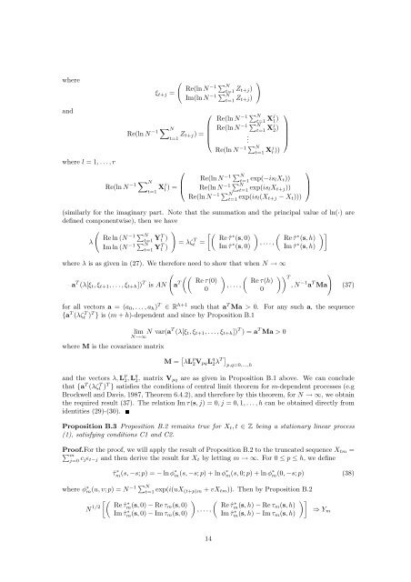
where λ is as given in (27). We therefore need to show that when N → ∞
( (( ) ( )) T
Re τ(0) Re τ(h)
a T (λ[ξ t , ξ t+1 , . . . , ξ t+h ]) T is AN a T , . . . ,
, N
0
0
−1 a Ma)
T
(37)
for all vectors a = (a 0 , . . . , a h ) T ∈ R h+1 such that a T Ma > 0. For any such a, the sequence
{a T (λζ T t )T } is (m + h)-dependent and since by Proposition B.1
where M is the covariance matrix
lim N
N→∞ var(aT (λ[ξ t , ξ t+1 , . . .,ξ t+h ]) T ) = a T Ma > 0
M = [ λL p 2 V pqL q 2 λT] p,q=0,...,h
and the vectors λ,L p 2 ,Lq 2 , matrix V pq are as given in Proposition B.1 above. We can conclude
that {a T (λζ T t ) T } satisfies the conditions of central limit theorem for m-dependent processes (e.g
Brockwell and Davis, 1987, Theorem 6.4.2), and therefore by this theorem, for N → ∞, we obtain
the required result (37). The relation Imτ(s, j) = 0, j = 0, 1, . . .,h can be obtained directly from
identities (29)-(30).
Proposition B.3 Proposition B.2 remains true for X t , t ∈ Z being a stationary linear process
(1), satisfying conditions C1 and C2.
Proof.For the proof, we will apply the result of Proposition B.2 to the truncated sequence X tm =
∑ m
j=0 c jǫ t−j and then derive the result for X t by letting m → ∞. For 0 ≤ p ≤ h, we define
ˆτ m ∗ (s, −s; p) = − lnφ∗ m (s, −s; p) + lnφ∗ m (s, 0; p) + lnφ∗ m (0, −s; p) (38)
where φ ∗ m(u, v; p) = N −1 ∑ N
t=1 exp(i(uX (t+p)m + vX tm )). Then by Proposition B.2
[( ) ( )]
N 1/2 Re ˆτ
∗
m (s, 0) − Re τ m (s, 0) Re ˆτ
∗
Im ˆτ m(s, ∗ , . . ., m (s, h) − Re τ m (s, h)
0) − Im τ m (s, 0) Im ˆτ m(s, ∗ ⇒ Y
h) − Im τ m (s, h) m
14