Estimating the Codifference Function of Linear Time Series Models ...
Estimating the Codifference Function of Linear Time Series Models ...
Estimating the Codifference Function of Linear Time Series Models ...
Create successful ePaper yourself
Turn your PDF publications into a flip-book with our unique Google optimized e-Paper software.
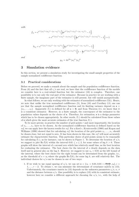
with<br />
{ f ij = e σα (|s i| α +|s j| α −|s i−s j| α ) 1 (|s i| α +|s j| α −|s i−s j| α) }<br />
2 eσα − 1<br />
+ e σα (|s i| α +|s j| α −|s i+s j| α ) { 1<br />
2 eσα (|s i| α +|s j| α −|s i+s j| α) − 1<br />
}<br />
+ 1<br />
{<br />
h ij = e σα (|s i| α +|s j| α −|s i−s j| α ) 1 (|s i| α +|s j| α −|s i−s j| α) }<br />
2 eσα − 1<br />
{ }<br />
+ e σα (|s i| α +|s j| α −|s i+s j| α )<br />
1 − 1 (|s i| α +|s j| α −|s i+s j| α )<br />
2 eσα<br />
and<br />
g ij = 4σ 2α |s i | α |s j | α<br />
3 Simulation evidence<br />
In this section, we present a simulation study for investigating <strong>the</strong> small sample properties <strong>of</strong> <strong>the</strong><br />
sample normalized codifference function.<br />
3.1 Practical considerations<br />
Before we proceed, we make a remark about <strong>the</strong> sample and <strong>the</strong> population codifference function.<br />
From (6) and <strong>the</strong> fact that all c j ’s are real, we have that <strong>the</strong> codifference function <strong>of</strong> <strong>the</strong> models<br />
we consider here is a real-valued function but <strong>the</strong> estimator (10) is complex. Therefore, one<br />
possibility is to use only <strong>the</strong> real part <strong>of</strong> <strong>the</strong> estimator. Because in practice we are working with a<br />
finite sample, <strong>the</strong> imaginary part <strong>of</strong> <strong>the</strong> estimator is still present, but will vanish asymptotically.<br />
In what follows, we are only working with <strong>the</strong> estimator <strong>of</strong> normalized codifference Î(k). Hence,<br />
we note that unlike <strong>the</strong> true normalized codifference (5), from (10) and Corollary 2.3, one can<br />
see that <strong>the</strong> sample normalized codifference function and its limiting variance depend on s =<br />
{s 1 , . . .,s r }. Apparently Î(·) is defined for all s > 0, and from Theorem 2.1, we know that it<br />
is a consistent estimator. However, in a finite sample, <strong>the</strong> convergence <strong>of</strong> <strong>the</strong> estimator to <strong>the</strong><br />
population values depends on <strong>the</strong> choice <strong>of</strong> s. Therefore, for estimation, s is a design parameter<br />
which has to be chosen appropriately. In o<strong>the</strong>r words, Î(·) should be calculated from those values<br />
<strong>of</strong> s which gives <strong>the</strong> most accurate estimates <strong>of</strong> <strong>the</strong> true function I(·).<br />
To be more precise, in practice <strong>the</strong> number <strong>of</strong> grid points r and more importantly, <strong>the</strong> location<br />
<strong>of</strong> s 1 , . . . , s r , have to be chosen. As <strong>the</strong> normalized codifference function is defined based on <strong>the</strong><br />
ecf, we can apply here <strong>the</strong> known results for ecf. For a fixed r, Koutrouvelis (1980) and Kogon and<br />
Williams (1998) showed that for calculating ecf, <strong>the</strong> location <strong>of</strong> <strong>the</strong> grid points s 1 , . . . , s r , should<br />
be chosen close, but not equal to zero. It has been shown in this case, <strong>the</strong> ecf will most accurately<br />
estimate <strong>the</strong> characteristic function. This particular choice <strong>of</strong> grid points seems to be reasonable<br />
for calculating Î(·), as for instance, can be shown in Figure 1. To determine <strong>the</strong> location <strong>of</strong> s i’s,<br />
we suggest to plot Re Î(k) within <strong>the</strong> interval 0.01 ≤ s ≤ 2, for some values <strong>of</strong> lag k > 0. These<br />
graphs will show <strong>the</strong> interval <strong>of</strong> s around zero which has relatively small bias, as <strong>the</strong> best location<br />
for evaluating <strong>the</strong> estimator. The best choice for <strong>the</strong> interval <strong>of</strong> s clearly depends on <strong>the</strong> data<br />
itself and in general also on <strong>the</strong> lag k. However, we suggest to use s a = 0.01 as <strong>the</strong> left bound <strong>of</strong><br />
<strong>the</strong> interval, where <strong>the</strong> best choice for <strong>the</strong> right bound can be determined from <strong>the</strong> graphs, i.e.,<br />
as <strong>the</strong> threshold <strong>of</strong> s = s b where <strong>the</strong> graphs Re Î(k), for some lag k, are still relatively flat. The<br />
individual choices for s i ’s can be chosen in one <strong>of</strong> two ways:<br />
1. If we wish to use equal spacing <strong>of</strong> s i ’s, we can set s = {s 1 = 0.01, 0.01 + i s b−s a<br />
r−1 , s b}, i =<br />
1, . . .,r − 2. To obtain r, we can minimize <strong>the</strong> determinant <strong>of</strong> covariance matrix in (13).<br />
Unfortunately, <strong>the</strong> covariance matrix in (13) depends on <strong>the</strong> unknown parameters c j ’s, α, σ<br />
and <strong>the</strong> distance between s i ’s. One possibility is to replace (13) with its consistent estimate,<br />
however here we consider a different approach for choosing <strong>the</strong> s i ’s, i.e., with <strong>the</strong> help <strong>of</strong><br />
5


