Estimating the Codifference Function of Linear Time Series Models ...

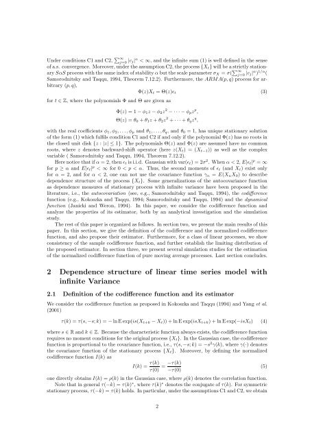
Under conditions C1 and C2, ∑ ∞
j=0 |c j| α < ∞, and the infinite sum (1) is well defined in the sense
of a.s. convergence. Moreover, under the assumption C2, the process {X t } will be a strictly stationary
SαS process with the same index of stability α but the scale parameter σ X = σ( ∑ ∞
j=0 |c j| α ) 1/α (
Samorodnitsky and Taqqu, 1994, Theorem 7.12.2). Furthermore, the ARMA(p, q) process for arbitrary
(p, q),
Φ(z)X t = Θ(z)ǫ t (3)
for t ∈ Z, where the polynomials Φ and Θ are given as
Φ(z) = 1 − φ 1 z − φ 2 z 2 − · · · − φ p z p ,
Θ(z) = θ 0 + θ 1 z + θ 2 z 2 + · · · + θ q z q ,
with the real coefficients φ 1 , φ 2 , . . . , φ p and θ 1 , . . .,θ q , and θ 0 = 1, has unique stationary solution
of the form (1) which fulfils condition C1 and C2 if and only if the polynomial Φ(z) has no roots in
the closed unit disk {z : |z| ≤ 1}. The polynomials Θ(z) and Φ(z) are assumed have no common
roots, where z denotes backward-shift operator (here z(X t ) = (X t−1 )) as well as the complex
variable ( Samorodnitsky and Taqqu, 1994, Theorem 7.12.2).
Here notice that if α = 2, then ǫ t is i.i.d. Gaussian with var(ǫ t ) = 2σ 2 . When α < 2, E|ǫ t | p = ∞
for p ≥ α and E|ǫ t | p < ∞ for 0 < p < α. Thus, the second moments of ǫ t (and X t ) exist only
for α = 2, and for α < 2, one can not use the covariance function γ n = E(X n X 0 ) to describe
dependence structure of the process {X t }. Some generalizations of the autocovariance function
as dependence measures of stationary process with infinite variance have been proposed in the
literature, i.e., the autocovariation (see, e.g., Samorodnitsky and Taqqu, 1994), the codifference
function (e.g., Kokoszka and Taqqu, 1994; Samorodnitsky and Taqqu, 1994) and the dynamical
function (Janicki and Weron, 1994). In this paper, we consider the codifference function and
analyze the properties of its estimator, both by an analytical investigation and the simulation
study.
The rest of this paper is organized as follows. In section two, we present the main results of this
paper. In this section, we give the definition of the codifference and the normalized codifference
function, and also propose their estimator. Furthermore, for a class of linear processes, we show
consistency of the sample codifference function, and further establish the limiting distribution of
the proposed estimator. In section three, we present several simulation studies for the estimation
of the normalized codifference function of pure moving average processes. Last section concludes.
2 Dependence structure of linear time series model with
infinite Variance
2.1 Definition of the codifference function and its estimator
We consider the codifference function as proposed in Kokoszka and Taqqu (1994) and Yang et al.
(2001)
τ(k) = τ(s, −s; k) = − ln E exp(is(X t+k − X t )) + ln E exp(isX t+k ) + ln E exp(−isX t ) (4)
where s ∈ R and k ∈ Z. Because the characteristic function always exists, the codifference function
requires no moment conditions for the original process {X t }. In the Gaussian case, the codifference
function is proportional to the covariance function, i.e., τ(s, −s; k) = −s 2 γ(k), where γ(·) denotes
the covariance function of the stationary process {X t }. Moreover, by defining the normalized
codifference function I(k) as
I(k) = τ(k)
τ(0) = −τ(k)
(5)
−τ(0)
one directly obtains I(k) = ρ(k) in the Gaussian case, where ρ(k) denotes the correlation function.
Note that in general τ(−k) = τ(k) ∗ , where τ(k) ∗ denotes the conjugate of τ(k). For symmetric
stationary process, τ(−k) = τ(k) holds. In particular, under the assumptions C1 and C2, we obtain
2