Estimating the Codifference Function of Linear Time Series Models ...
Estimating the Codifference Function of Linear Time Series Models ...
Estimating the Codifference Function of Linear Time Series Models ...

You also want an ePaper? Increase the reach of your titles
YUMPU automatically turns print PDFs into web optimized ePapers that Google loves.
(and similarly for <strong>the</strong> imaginary part), where φ ∗ (u, v; j) = N −1 ∑ N<br />
t=1 exp(i(uX t+j+vX t )), φ(u, v; j)=<br />
(N − j) −1 ∑ N−j<br />
t=1 exp(i(uX t+j + vX t )) and λ 2 = [ −1 1 1 ] . The required result <strong>the</strong>n follows<br />
from Slutzky’s <strong>the</strong>orem (e.g., Theorem 5.1.1. in Lehmann, 1999).<br />
Simple algebra gives, for 0 ≤ j ≤ h,<br />
⎛<br />
N 1/2 E<br />
∣ λ 2<br />
⎝ Re ⎞ ⎛<br />
φ∗ (s k , −s k ; j)<br />
Reφ ∗ (s k , 0; j) ⎠ − λ 2<br />
⎝ Re φ(s ⎞<br />
k, −s k ; j)<br />
Re φ(s k , 0; j) ⎠<br />
Re φ ∗ (0, −s k ; j) Reφ(0, −s k ; j) ∣<br />
⎛ j<br />
∑<br />
1 N (N−j) N t=1<br />
= N 1/2 E<br />
λ ⎜<br />
cos(is k(X t+j − X t )) − 1 ∑ N<br />
N−j t=N−j+1 cos(is(X ⎞<br />
t+j − X t ))<br />
j<br />
∑<br />
1 N 2 ⎝ (N−j) N t=1 cos(is kX t+j ) − 1 ∑ N<br />
N−j t=N−j+1 cos(is ⎟<br />
kX t+j ) ⎠<br />
∣<br />
j 1<br />
∑ N<br />
(N−j) N t=1 cos(−is kX t )) − 1 ∑ N<br />
N−j t=N−j+1 cos(−is kX t ) ∣<br />
≤ 6j(N − j) −1/2 ( N<br />
N−j )1/2<br />
The required result is obtained from 3j(N − j) −1/2 → 0 and N/(N − j) → 1 as N → ∞. Using<br />
<strong>the</strong> same arguments, similar results can be obtained for <strong>the</strong> imaginary part. The conclusion <strong>of</strong> <strong>the</strong><br />
<strong>the</strong>orem <strong>the</strong>n follows from Proposition B.3 above.<br />
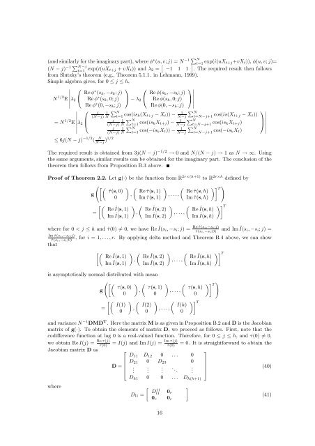
Pro<strong>of</strong> <strong>of</strong> Theorem 2.2. Let g(·) be <strong>the</strong> function from R 2r×(h+1) to R 2r×h defined by<br />
( [( ) ( ) ( )] ) T<br />
ˆτ(s, 0) Re ˆτ(s, 1) Re ˆτ(s, h)<br />
g<br />
,<br />
, . . . ,<br />
0 Im ˆτ(s, 1) Im ˆτ(s, h)<br />
[( ) ( ) ( )] T<br />
Re Î(s, 1) Re Î(s, 2) Re Î(s, h)<br />
=<br />
Im Î(s, 1) ,<br />
Im Î(s, 2) , . . .,<br />
Im Î(s, h)<br />
where for 0 < j ≤ h and ˆτ(0) ≠ 0, we have Re Î(s Re ˆτ(si,−si;j)<br />
i, −s i ; j) =<br />
ˆτ(s i,−s i;0)<br />
and ImÎ(s i, −s i ; j) =<br />
Im ˆτ(s i,−s i;j)<br />
ˆτ(s i,−s i;0)<br />
, for i = 1, . . .,r. By applying delta method and Theorem B.4 above, we can show<br />
that<br />
[( ) ( ) ( )] T<br />
Re Î(s, 1) Re Î(s, 2) Re Î(s, h)<br />
Im Î(s, 1) ,<br />
Im Î(s, 2) , . . . ,<br />
Im Î(s, h)<br />
is asymptotically normal distributed with mean<br />
( [( ) (<br />
τ(s, 0) τ(s, 1)<br />
g<br />
,<br />
0 0<br />
[( ) ( I(1) I(2)<br />
= ,<br />
0 0<br />
)<br />
, . . . ,<br />
) (<br />
τ(s, h)<br />
, . . . ,<br />
0<br />
( I(h)<br />
0<br />
)] T<br />
)] T<br />
)<br />
and variance N −1 DMD T . Here <strong>the</strong> matrix M is as given in Proposition B.2 and D is <strong>the</strong> Jacobian<br />
matrix <strong>of</strong> g(·). To obtain <strong>the</strong> elements <strong>of</strong> matrix D, we proceed as follows. First, note that <strong>the</strong><br />
codifference function at lag 0 is a real-valued function. Therefore, for 0 ≤ j ≤ h, and τ(0) ≠ 0,<br />
we obtain Re I(j) =<br />
Jacobian matrix D as<br />
where<br />
Re τ(j)<br />
τ(0)<br />
= I(j) and ImI(j) =<br />
Im τ(j)<br />
τ(0)<br />
⎡<br />
⎤<br />
D 11 D 12 0 . . . 0<br />
D 21 0 D 23 0<br />
D = ⎢<br />
⎣<br />
.<br />
.<br />
.<br />
. .. .<br />
⎥<br />
⎦<br />
D h1 0 0 . . . D h(h+1)<br />
[ ]<br />
D<br />
11<br />
D l1 =<br />
l1<br />
0 r<br />
0 r 0 r<br />
= 0. It is straightforward to obtain <strong>the</strong><br />
(40)<br />
(41)<br />
16