Chapter 4: Programming in Matlab - College of the Redwoods

4 Programming In Matlab 

In this chapter, we study the fundamentals of programming in Matlab. We begin 

with a study of logical arrays and the operators and method that make them so 

effective in Matlab programming. 

Table of Contents 

4.1 Logical Arrays . . . . . . . . . . . . . . . . . . . . . . . . . . . . . . . . . . . . . . . . . . . . . . 261 

Relational Operators 263 

How Logical Arrays are Used 265 

Logical Operators 277 

Exercises 285 

Answers 289 

4.2 Control Structures in Matlab . . . . . . . . . . . . . . . . . . . . . . . . . . . . . . . . . 299 

If 299 

Else 300 

Elseif 301 

Switch, Case, and Otherwise 304 

Loops 306 

For k = A 311 

Break and Continue 312 

Any and All 314 

Nested Loops 316 

Fourier Series — An Application of a For Loop 318 

Exercises 323 

Answers 327 

4.3 Functions in Matlab . . . . . . . . . . . . . . . . . . . . . . . . . . . . . . . . . . . . . . . . . 333 

Anonymous Functions 333 

Function M-Files 338 

More Than One Output 343 

No Output 346 

Exercises 349 

Answers 353 

4.4 Variable Scope in Matlab . . . . . . . . . . . . . . . . . . . . . . . . . . . . . . . . . . . . 361 

The Base Workspace 361 

Scripts and the Base Workspace 362 

Function Workspaces 364 

Global Variables 368 

Persistent Variables 369 

Exercises 372 

Answers 377

260 Chapter 4 Programming In Matlab 

4.5 Subfunctions in Matlab . . . . . . . . . . . . . . . . . . . . . . . . . . . . . . . . . . . . . . 379 

Calling Functions From Script Files 380 

Subfunctions 383 

Adding Functionality to our Program 385 

Completing rationalArithmetic.m 391 

Exercises 393 

4.6 Nested Functions in Matlab . . . . . . . . . . . . . . . . . . . . . . . . . . . . . . . . . . 399 

Variable Scope in Nested Functions 400 

Graphical User Interfaces 403 

Button Groups and Radio Buttons 406 

Adding a Function Callback to the UIButtonGroup 409 

Popup Menus 411 

Edit Boxes 415 

Appendix 418 

Exercises 422 

Answers 430 

Copyright 

All parts of this Matlab Programming textbook are copyrighted in the name 

of Department of Mathematics, College of the Redwoods. They are not in 

the public domain. However, they are being made available free for use 

in educational institutions. This offer does not extend to any application 

that is made for profit. Users who have such applications in mind should 

contact David Arnold at david-arnold@redwoods.edu or Bruce Wagner at 

bruce-wagner@redwoods.edu. 

This work (including all text, Portable Document Format files, and any other 

original works), except where otherwise noted, is licensed under a Creative 

Commons Attribution-NonCommercial-ShareAlike 2.5 License, and is copyrighted 

C○2006, Department of Mathematics, College of the Redwoods. To 

view a copy of this license, visit http://creativecommons.org/licenses/by-ncsa/2.5/ 

or send a letter to Creative Commons, 543 Howard Street, 5th Floor, 

San Francisco, California, 94105, USA.

Section 4.1 Logical Arrays 261 

4.1 Logical Arrays 

We begin this section by demonstraing how Matlab determines the truth or 

falsehood of a statement. Enter the following array at the Matlab prompt. 

>> x=[true false] 

x = 

1 0 

Note that that true evaluates to 1, while false evaluates to zero. Moreover, the 

array stored in the variable x in an entirely new type of datatype, called a logical 

array. 

>> whos 

Name Size Bytes Class 

x 1x2 2 logical array 

Note that each entry in the logical vector x takes one byte of storage. Note that 

this logical type is a completely new datatype. Indeed, it is instructive to compare 

the vector x with the following vector y 

>> y=[1 0] 

y = 

1 0 

On the surface, it appears that the variables x and y contain exactly the same 

data, that is until one checks the datatypes with Matlab’s whos command. 

>> whos 


x 1x2 2 logical array 

y 1x2 16 double array 

1 Copyrighted material. See: http://msenux.redwoods.edu/Math4Textbook/

262 Chapter 4 Programming in Matlab 

Note that vector y is of class double, using 8 bytes to store each entry. 

Alternatively, we can check the class with Matlab’s class command. On the 

one hand, the command 

>> class(x) 

ans = 

logical 

informs us that vector x has class logical. On the other hand, the command 

>> class(y) 

ans = 

double 

informs us that the vector y has class double. 

Like some of the other conversion operators we’ve seen (like uint8), Matlab 

provides an operator that will convert numeric arrays to logical arrays. Any 

nonzero real number is converted to a logical 1 (true) and zeros are converted to 

logical 0 (false). 

To see this in action, first enter the following matrix A. 

>> A=[0 1 3;4 0 0; 5 7 -11] 

A = 

0 1 3 

4 0 0 

5 7 -11 

Note that A has class double. 

>> class(A) 

ans = 

double 

Now, convert A to a logical array.


>> A=logical(A) 

Warning: Values other than 0 or 1 converted to logical 1. 

A = 

0 1 1 

1 0 0 

1 1 1 

Note that all nonzero entries in the original matrix A are now logical 1, while all 

zeros in the original matrix A are now logical zero. You can test the new class of 

matrix A with the following command. 

>> class(A) 

ans = 

logical 

Relational Operators 

Matlab provides a complete list of relational operators (see Table 4.1). 

Operator 

Description 

< Less than 

≤ 

Less than or equal to 

> Greater than 

≥ 

Greater than or equal to 

== Equal to 

∼= Not equal to 

Table 4.1. Matlab’s 

relational operators. 

The Matlab relational operators compare corresponding elements of arrays with 

equal dimensions. Relational operators always operate element-by-element. That 

is, they are “array smart.” 

For example, consider the vectors v and w.


>> v=[1 3 6] 

v = 

1 3 6 

>> w=[1 2 4] 

w = 

1 2 4 

The output of the command v>w will return a logical vector of the same size as 

the vectors v and w. Locations where the specified relation is true receive a 1 

and locations where the specified relation is false receive a 0. 

>> v>w 

ans = 

0 1 1 

Because the first entry of v is not larger than the first entry of w, the first entry 

of the answer receives a zero (false). Because the second and third entries of the 

vector v are larger than the second and third entries of the vector w, the second 

and third entries of the answer receive a 1 (true). This is what we mean when we 

say “Relational operators always operate element-by-element.” 

Like the other array operators we’ve seen that act in an element-by-elemnt 

manner, the arrays being compared must have the same size. 

>> u=[10 10] 

u = 

10 10 

>> u>v 

??? Error using ==> gt 

Matrix dimensions must agree. 

Comparing with a scalar. One exception to the “same size rule” is when 

an array is compared to a scalar. In this case, Matlab tests the scalar against 

every element of the other operand.


>> u=rand(1,6) 

u = 

0.9501 0.2311 0.6068 0.4860 0.8913 0.7621 

>> u>0.5 

ans = 

1 0 1 0 1 1 

Note that the first, third, fifth, and sixth entries of the vector u are all greater 

than 0.5, so the answer receives a 1 (true) in these positions, with the remaining 

positions receiving a 0 (false). 

How Logical Arrays are Used 

Matlab uses logical arrays for a type of indexing. A logical index designates the 

elements of a matrix A based on their position in the indexing array, B. In this 

masking type of operation, every true element in the indexing array is treated as 

a positional index into the array being accessed 

For example, create a matrix A of uniform random numbers. 

>> A=rand(5) 

A = 

0.4565 0.7919 0.9355 0.3529 0.1987 

0.0185 0.9218 0.9169 0.8132 0.6038 

0.8214 0.7382 0.4103 0.0099 0.2722 

0.4447 0.1763 0.8936 0.1389 0.1988 

0.6154 0.4057 0.0579 0.2028 0.0153 

Next, find the positions of the random numbers that are less than 0.5, and store 

the result in the matrix B. 

>> B=A


Take a moment to check that in each position in B that contains a logical 1 (true), 

the corresponding position in matrix A contains a uniform random number that 

is less than 0.5. 

There are a number of things that we can do with this information. We could 

list all the random numbers in A that are less than 0.5 by using matrix B as a 

logical index into the matrix A. 2 

>> A(B) 

ans = 

0.4565 

0.0185 

0.4447 

0.1763 

0.4057 

0.4103 

0.0579 

0.3529 

0.0099 

0.1389 

0.2028 

0.1987 

0.2722 

0.1988 

0.0153 

Or we could set each of these positions to zero. 

>> A(B)=0 

A = 

0 0.7919 0.9355 0 0 

0 0.9218 0.9169 0.8132 0.6038 

0.8214 0.7382 0 0 0 

0 0 0.8936 0 0 

0.6154 0 0 0 0 

2 Matlab has roots that began their growth in Fortran, where the entries in arrays were loaded 

by column. The Matlab command A(:) will list all the entries in A, first going down the 

first column, then the second, etc. With the command A(B), Matlab first lists all the “true” 

positions in the first column, then the second, etc.


A number of Matlab’s functions are designed to execute a test of some sort, 

then return a logical array. The output of these commands is usually used as a 

mask or index. For example, create a magic square with the following command. 

>> A=magic(5) 

A = 

17 24 1 8 15 

23 5 7 14 16 

4 6 13 20 22 

10 12 19 21 3 

11 18 25 2 9 

We’ll find all the primes in matrix A with Matlab’s ispime command. 

>> B=isprime(A) 

B = 

1 0 0 0 0 

1 1 1 0 0 

0 0 1 0 0 

0 0 1 0 1 

1 0 0 1 0 

Each position in matrix B that contains a logical 1 (true) indicates a prime in the 

corresponding position of matrix A. We can get a listing of the primes in matrix 

A. 

>> A(B) 

ans = 

17 

23 

11 

5 

7 

13 

19 

2 

3


Or we can replace all of the primes in Matrix A with −1 with this command. 

>> A(B)=-1 

A = 

-1 24 1 8 15 

-1 -1 -1 14 16 

4 6 -1 20 22 

10 12 -1 21 -1 

-1 18 25 -1 9 

A Practical Example. Although the examples provided thus far provide 

explanation on how logical arrays are used as indices, they might not seem to 

have much practical use. Let’s look at some examples where logical indexing is 

helpful in a much more practical way. 

◮ Example 1. Plot the graph of y = √ x 2 − 1 over the interval [−5, 5]. 

Seems like a simple request. 

>> x=linspace(-5,5,100); 

>> y=sqrt(x.^2-1); 

>> plot(x,y) 

Figure 4.1. 

y = √ x 2 − 1. 

Plotting of the graph of


Seems to have worked (see Figure 4.1(a)), but we do receive a warning at the 

command line when we run this script. 

Warning: Imaginary parts of complex X and/or Y arguments ignored 

Complex numbers have seemingly crept into our calculations. They certainly 

don’t exist in the vector x, because the command x=linspace(-5,5,200) generates 

real numbers between −5 and 5. It must be the vector y that contains the 

complex numbers, but how to find them? 

Real and imaginary parts of complex numbers. A complex number has 

the form a + bi, where i = √ −1. The real part of the complex number a + bi is 

the number a. The imaginary part of the complex number a + bi is the number 

b. Matlab know all about the real and imaginary parts of complex numbers. 

First, check that the variable i contains the complex number i. We do this 

because i is a popular variable to use in scripts and for loops and may have been 

set to something other than the complex number i. 

>> i 

ans = 

0 + 1.0000i 

If you don’t get this result, type clear i and try again. 

Enter z = 3 + 4i. 

>> z=3+4i 

z = 

3.0000 + 4.0000i 

The real part of z = 3 + 4i is 3. 

>> real(z) 

ans = 

3 

The imaginary part of z = 3 + 4i is 4.


>> imag(z) 

ans = 

4 

Now, a number r is real if and only if the real part of r is identical to the number 

r. For example, set r = 4. 

>> r=4 

r = 

4 

Now test if its real part is identical to itself. 

>> real(r)==r 

ans = 

1 

Note that the logical 1 indicates a “true” response. The real part of r equals r. 

Thus, r is a real number. 

On the other hand, set z = 2 − 3i. 

>> z=2-3i 

z = 

2.0000 - 3.0000i 

Test if the real part of z equals z. 

>> real(z)==z 

ans = 

0 

Note that the logical 0 indicates a “false” response. The real part of z doesn’t 

equal z. Thus, z is not a real number, z is complex. 

Let’s use this idea to find the positions in the vector y that hold complex 

numbers.


>> k=real(y)~=y 

k = 

Columns 1 through 10 

0 0 0 0 0 0 0 0 0 0 


0 0 0 0 0 0 0 0 0 0 


0 0 0 0 0 0 0 0 0 0 


0 0 0 0 0 0 0 0 0 0 


1 1 1 1 1 1 1 1 1 1 


1 1 1 1 1 1 1 1 1 1 


0 0 0 0 0 0 0 0 0 0 


0 0 0 0 0 0 0 0 0 0 


0 0 0 0 0 0 0 0 0 0 


0 0 0 0 0 0 0 0 0 0 

The vector k is a logical vector, having logical 1 (true) in each position that y 

has a complex number. We can use this as an index into the vector x to see what 

values of x are causing complex numbers to appear in the vector y. 

>> x(k) 

ans = 


-0.9596 -0.8586 -0.7576 -0.6566 -0.5556 -0.4545 


-0.3535 -0.2525 -0.1515 -0.0505 0.0505 0.1515 


0.2525 0.3535 0.4545 0.5556 0.6566 0.7576 


0.8586 0.9596 

It would appear that values of x between −1 and 1 are creating complex values in 

the vector y. This makes sense because the domain of the function y = √ x 2 − 1


requires that x 2 − 1 ≥ 0. Solving for x, |x| ≥ 1, or equivalently, x ≤ −1 or 

x ≥ 1. For values of x between −1 and 1, the expression x 2 − 1 is negative, so 

the square root produces complex numbers. We can see the complex numbers in 

y with logical indexing. 

>> y(k) 

ans = 


0 + 0.2814i 0 + 0.5127i 0 + 0.6527i 


0 + 0.7543i 0 + 0.8315i 0 + 0.8907i 


0 + 0.9354i 0 + 0.9676i 0 + 0.9885i 


0 + 0.9987i 0 + 0.9987i 0 + 0.9885i 


0 + 0.9676i 0 + 0.9354i 0 + 0.8907i 


0 + 0.8315i 0 + 0.7543i 0 + 0.6527i 


0 + 0.5127i 0 + 0.2814i 

Note that the real part of each of these complex numbers is zero. 

So, how does Matlab’s plot command handle complex numbers. The answer 

is found by typing help plot. The relevant part of the helpfile follows. 

PLOT(Y) plots the columns of Y versus their index. 

If Y is complex, PLOT(Y) is equivalent to 

PLOT(real(Y),imag(Y)). In all other uses of PLOT, 

the imaginary part is ignored. 

In the case at hand, we used plot(x,y), so this paragraph of the help file for the 

plot command would indicate that Matlab simply ignores the imaginary parts 

of the vector y when the entries are complex. For the output of y(k) above, 

when Matlab ignores the imaginary part, that is equivalent to saying that Matlab 

considers all of these complex numbers to equal their real part, or zero. This 

can be seen by adding the command axis([-5,5,-5,5]) to produce the image in 

Figure 4.2.


>> axis([-5,5,-5,5]) 

Figure 4.2. The axis command reveals 

that the plot command believes 

that all y-values equal zero for values of 

x between −1 and 1. 

Note the horizontal line connecting the right- and left-hand halves of the hyperbola 

in Figure 4.2. This line simply does not belong in this image, as x-values between 

−1 and 1 are not in the domain of of y = √ x 2 − 1. However, Matalb simply 

ignores the imaginary part of the complex numbers in the vector y, considers 

them to be zero, and plots this “false” horizontal line. 

Let’s get rid of this “false” horizontal line by setting all the offending complex 

number entries in the vector y to NaN (Matlab’s “Not a Number.”) 

>> y(k)=NaN; 

If you remove the suppressing semicolon at the end of this command, you will be 

able to see that all the complex numbers in the vector y have been replaced by 

NaN. 

The good news is the fact that Matlab’s plot command ignores these NaN’s 

and does not plot them. The following command will produce the image in 

Figure 4.3.


>> plot(x,y) 

>> axis([-5,5,-5,5]) 

Figure 4.3. Removing the complex 

numbers from the plot. 

Preplanning. All of these contortions with complex numbers can be avoided 

with proper preplanning. As we’ve said, the domain of y = √ x 2 − 1 is {x : x ≤ 

−1 or x ≥ 1}. 

We’ll start by defining an anonymous function, making it “array smart.” 

>> f=@(x) sqrt(x.^2-1) 

f = 

@(x) sqrt(x.^2-1) 

Test the anonymous function at x = 0, where f(0) = √ 0 2 − 1 = √ −1 = i. 

>> f(0) 

ans = 

0 + 1.0000i 

Note that f(0) = i is a correct response. 

We’ll first plot the left-hand branch of the hyperbola on {x : x ≤ −1}.


>> x=linspace(-5,-1); 

>> y=f(x); 

>> plot(x,y) 

Because each of the entries in the vector x lie in the domain of the function 

y = √ x 2 − 1, no complex numbers are produced when evaluating the function on 

the entries in x. 

Next, we’ll plot the right-hand branch of the hyperbola on {x : x ≥ 1}. Again, 

no complex numbers are produced because we are using x-values that lie in the 

domain of the function. 

>> x=linspace(1,5); 

>> y=f(x); 

>> line(x,y) 

Remember that the line command is used to append to an existing plot. We 

could also have used a hold on, followed by a plot(x,y), but the line command 

does not require that we “hold” the plot. 

Finally, adjust the window boundaries with the axis command. 

>> axis([-5,5,-5,5]) 

The result is an image indentical to that in Figure 4.3. 

Complex numbers are not so easily avoided in other situations. Let’s look at 

an example that uses Matlab’s mesh command. 

◮ Example 2. Sketch the surface z = √ x 2 − y 2 on the rectangular domain 

D = {(x, y) : −2 ≤ x, y ≤ 2}. 

Let’s again use an anonymous function, making it “array smart.” 

>> f=@(x,y) sqrt(x.^2-y.^2) 

f = 

@(x,y) sqrt(x.^2-y.^2)


Test the anonymous function. Note that f(5, 3) = √ 5 2 − 3 2 = 4. 

>> f(5,3) 

ans = 

4 

That looks correct. 

Now, the following commands produce the image in Figure 4.4(a). At first 

glance, it appears that all is well. 

>> [x,y]=meshgrid(linspace(-2,2,50)); 

>> z=f(x,y); 

>> mesh(x,y,z) 

However, this time Matlab ignores the imaginary part of the complex numbers in 

z without even providing a warning. This is evident in the graph of z = √ x 2 − y 2 

where you see that a large number of points in the mesh have z-value equal to 

zero. These points in the xy-plane are where Matlab is ignoring the imaginary 

part of the complex entries in z and plotting only the real part (which is zero). 

We can check to see if the matrix z contains any complex numbers. 

>> isreal(z) 

ans = 

0 

The false response indicates the presence of complex numbers in matrix z. We 

can replace all the complex entries in z with these commands. 

>> k=real(z)~=z; 

>> z(k)=NaN; 

You may want to remove the suppressing semicolons and view the output of the 

last two commands. 

Matlab’s mesh command refuses to plot the Nan’s and produces the image 

in Figure 4.4(b).


>> mesh(x,yz) 

(a) 

(b) 

Figure 4.4. Removing the complex 

entries removes the false zero plane. 

Logical Operators 

The Matlab symbols &, |, and ~ are the logical operators AND, OR, and NOT, 

respectively. Truth tables for each logical operator are gathered in Table 4.2. 

Remember that logical 1 is true and logical 0 is false. 

• The statment “A and B” is true if and only if both statements A and B are 

true. This is reflected in the truth table for & (AND) in Table 4.2(a). 

• The statement “A or B” is true if and only if one or the other of statements A 

and B are true. This is reflected in te truth table for | (OR) in Table 4.2(b). 

• The statement “not A” simply reverses the truth or falsehood of statement A. 

This is reflected in the truth table for ∼ (NOT) in Table 4.2(c). 

Each of the logical operators &, |, and ~ acts element-wise. Moreover, the 

output is of type logical. For example, create two logical vectors u and v. 

>> u=logical([1 1 1 0 0]); 

>> v=logical([1 0 1 0 1]);


A B A & B 

1 1 1 

1 0 0 

0 1 0 

0 0 0 

A B A | B 

1 1 1 

1 0 1 

0 1 1 

0 0 0 

A 

∼ A 

1 0 

0 1 

(a) AND (b) OR (c) NOT 

Table 4.2. 

Truth tables for Matlab’s logical operators. 

The first and third entries of vectors u and v are logical 1’s (true), hence the 

first and third entries of u&v will be logical 1’s (true). According to Table 4.2(a), 

all other entries of u&v will be logical 0’s (false). 

>> u, v, u&v 

u = 

1 1 1 0 0 

v = 

1 0 1 0 1 

ans = 

1 0 1 0 0 

On the other hand, Table 4.2(b) indicates that u|v (OR) will be false if and 

only if both entries are false. In the case of the vectors u and v, the fourth entry 

of each vector is logical 0 (false), so the fourth entry of u|v will be logical 0 (false). 

All other entries of u|v will be logical 1’s (true). 

>> u, v, u|v 

u = 

1 1 1 0 0 

v = 

1 0 1 0 1 

ans = 

1 1 1 0 1 

u. 

Finally, ~u simply reverses the truth or falsehood of each entry of the vector


>> u, ~u 

u = 

1 1 1 0 0 

ans = 

0 0 0 1 1 

If the vectors and/or matrices involved are not logical arrays, the logical operators 

first convert the operands to logical arrays. First, create a “magic” matrix 

A. 

>> A=magic(3) 

A = 

8 1 6 

3 5 7 

4 9 2 

Create a diagonal matrix D with the vector [5, 6, 7] on its main diagonal. 

>> D=diag([5,6,7]) 

D = 

5 0 0 

0 6 0 

0 0 7 

We could first convert these to logical matrices and then “and” them.


>> LA=logical(A), LD=logical(D), LA&LD 


LA = 

1 1 1 

1 1 1 

1 1 1 


LD = 

1 0 0 

0 1 0 

0 0 1 

ans = 

1 0 0 

0 1 0 

0 0 1 

However, this is not necessary, because the operator & will convert each of its 

operands to a logical type before performing the AND operation. 

>> A, D, A&D 

A = 

8 1 6 

3 5 7 

4 9 2 

D = 

5 0 0 

0 6 0 

0 0 7 

ans = 

1 0 0 

0 1 0 

0 0 1 

Finally, because the logical operators act element-wise, the arrays used as 

operands must have the same dimensions.


>> u=[2,3], v=[4 5 6], u|v 

u = 

2 3 

v = 

4 5 6 

??? Error using ==> or 

Inputs must have the same size. 

Let’s look at some powerful applications of these operators. 

◮ Example 3. 

Find all entries of matrix magic(5) that are not prime. 

Start by entering the matrix and using Matlab’s isprime function to find the 

prime entries. 

>> M=magic(5); B=isprime(M); 

We saw in an earlier example that M(B) will list all of the primes in the matrix 

M. So, let’s use the logical operator ~ to list all the nonprimes. For convenience 

and purposes of comparison, we list the matrix M. 

>> M 

M = 

17 24 1 8 15 

23 5 7 14 16 

4 6 13 20 22 

10 12 19 21 3 

11 18 25 2 9 

Now we list all the nonprimes in the matrix M.


>> M(~B) 

ans = 

4 

10 

24 

6 

12 

18 

1 

25 

8 

14 

20 

21 

15 

16 

22 

9 

Even more succinctly, try the command M(~isprime(M)) to achieve the same 

result. 

Let’s look at another example. 

◮ Example 4. Sketch the surface z = x 2 + y 2 on the rectangular domain 

d = {(x, y) : −1 ≤ x, y ≤ 1}, but only for those pairs (x, y) that satisfy y < x 

and y > −x. 

Let’s again use an anonymous function, making it “array smart.” 

>> f=@(x,y) x.^2+y.^2 

f = 

@(x,y) x.^2+y.^2 

Test the function. Note that f(3, 4) = 3 2 + 4 2 = 25. 

>> f(3,4) 

ans = 

25


That checks. 

Next, create the rectangular grid and evaluate z at each point (x, y) in the 

grid. 

[x,y]=meshgrid(linspace(-1,1,50)); 

z=f(x,y); 

Now, find those values of the grid that satisfy y < x and y > −x. 

k=(y-x); 

We want to eliminate from the mesh all points that do not satisfy this requirement. 

z(~k)=NaN; 

We can now draw the resulting mesh, label the axes, and provide an orientation. 

mesh(x,y,z) 

xlabel(’x-axis’) 

ylabel(’y-axis’) 

zlabel(’z-axis’) 

box on 

view(145,20) 

The result is shown in Figure 4.5(a). 

An interesting view is provided by the following command, the result of which 

is shown in Figure 4.5(b). In this view, we’ve declined to rotate the xy-axes, but 

elevated our eye 90 ◦ , so that we are gazing directly down at the xy-plane. This 

view clearly shows that we have sketched the surface of a region in the rectangular 

domain restricted to (x, y) pairs satisfying y < x and y > −x. 

view(0,90)


Figure 4.5. 

y > −x. 

(a) 

The surface z = x 2 + y 2 restricted to points where y < x and 

(b)


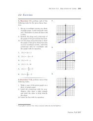
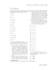
4.1 Exercises 

In Exercises 1-6, first enter the following 

vectors. 

>> v=[1,3,5,7], w=[5,2,5,4] 

v = 

1 3 5 7 

w = 

5 2 5 4 

In each exercise, first predict the output 

of the given command, then validate 

your response with the appropriate 

Matlab command. Note: The 

idea here is not to simply enter the 

command. Rather, spend some time 

thinking, then predict the output before 

you enter the command to verify 

your conclusion. 

1. v>w 

2. v>=w 

3. v A=magic(5) 

A = 

17 24 1 8 15 

23 5 7 14 16 

4 6 13 20 22 

10 12 19 21 3 

11 18 25 2 9 

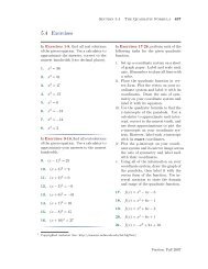
In Exercises 7-12, first predict the 

output of the given command, then 

validate your response with the appropriate 

Matlab command. Note: The 

idea here is not to simply enter the 

command. Rather, spend some time 

thinking, then predict the output before 

you enter the command to verify 

your conclusion. 

7. 

8. 

9. 

>> A>14 

>> A> (A>3) & (A


11. 

12. 

>> (A=21) 

>> ~(A> (A>6) & ~(A>8) 

13. Set P=pascal(5). Write a Matlab 

command that will list all entries 

of matrix P that are less than 20 but 

not equal to 1. 



of matrix P that are not equal to 1. 



of matrix P that are less than or equal 

to 4 or greater than 20. 



of matrix P that are greater than 3 

but not greater than 35. 

When a and b are positive integers, 

the Matlab command mod(a,b) returns 

the remainder when a is divided 

by b. Use this command to produce 

the requested entries of the given matrix 

in Exercises 17-20. 

17. Set A=magic(4). Write a Matlab 

command that will return all entries 

of matrix A that are divisible by 

2. Hint: An integer k is divisible by 

2 if the remainder is zero when k is 

divided by 2. 



of matrix A that are odd integers. 

Hint: A integer k is odd if its 

remainder is 1 when k is divided by 2. 




3. 




5. 

21. Execute the following command 

to list the primes less than or equal to 

100. 

>> primes(100) 

Secondly, create a vector u holding 

the integers from 1 to 100, inclusive. 

Use Matlab’s isprime command 

and logical indexing to pick out and 

list all the primes in vector u. Compare 

the results. 

22. Create a vector u holding the 

integers from 100 to 1000, inclusive. 

Use Matlab’s isprime command and 

logical indexing to pick out all the primes 

in vector u. Use Matlab’s max command 

on the result to find the largest


prime between 100 and 1000. 

In Exercises 23-26, perform each of 

the following tasks for the given function. 

i. Write an “array smart” anonymous 

function f for the given function. 

Test your anonymous function before 

proceeding. 

ii. Set x=linspace(-10,10,200) and 

evaluate the function with y=f(x). 

iii. Use the plot(x,y) command to plot 

the function. 

iv. Use axis([-10,10,-10,10]) to set 

the window boundaries. 

v. Use logical indexing to set all of 

the complex entries in the vector 

y to NaN. Open a second figure 

window with the command figure. 

Replot the result and reset the window 

boundaries as above, if necessary. 

Add axis labels and a title 

and turn the grid on. 

23. f(x) = 2 + √ x + 5 

24. f(x) = 3 − √ x − 3 

25. f(x) = √ 9 − x 2 

26. f(x) = √ x 2 − 25 

In Exercises 27-30, use “advanced 

planning” to plot the given function 

on a subset of the domain [−10, 10] 

to avoid complex entries when evaluating 

the given function. In each 

case, set the window boundaries with 

the command axis([-10,10,-10,10]), 

turn on the grid, and add axes labels 

and a title. 

27. The function in Exercise 23. 





the following tasks for the given function. 





ii. Set: 

x=linspace(-3,3,40); 

y=x; 

[x,y]=meshgrid(x,y); 

Evaluate the function with z=f(x,y). 

iii. Use mesh(x,y,z) to plot the surface 

defined by the function. 

iv. Use logical indexing to set all of 

the complex entries in the vector 

z to NaN. Open a second figure 

window with the command figure. 

Replot the surface. Add axis labels 

and a title. 

31. f(x, y) = √ 1 + x 

32. f(x, y) = √ 1 − y 

33. f(x, y) = √ 9 − x 2 − y 2 

34. f(x, y) = √ x 2 + y 2 − 1 


the following tasks for the given func-


tion. 





ii. Set: 

39. f(x, y) = 11 − 2x + 2y where 

x + y < 0 and x ≥ −2. 

40. f(x, y) = 10 + 2x − 3y where 

x − 2y ≤ 0 or y ≤ 0. 


y=x; 


Evaluate the function with z=f(x,y). 

iii. Use logical indexing to replace all 

entries in z with NaN that do not 

satisfy the given constraint. 

iv. Use mesh(x,y,z) to plot the surface 

defined by the function and 

constraint. Add axis labels and a 

title. 

v. Open a second figure window with 

the command figure. Replot the 

surface and orient the view with 

view(0,90). Add axis labels and 

a title. Does the pictured region 

satisfy the given constraint? 

35. f(x, y) = 12 − x − y where 

x > −1. 

36. f(x, y) = 10 − 2x + y where 

y ≤ 3. 

37. f(x, y) = 14 + x − 2y where 

x + y < 0. 

38. f(x, y) = 14 + x − 2y where 

x − y ≥ 0.


4.1 Answers 

1. 

3. 

5. 

>> v>w 

ans = 

0 1 0 1 

>> v> v==w 

ans = 

0 0 1 0 

11. 

13. 

>> (A>3) & (A> ~(A> A>14 

ans = 

1 1 0 0 1 

1 0 0 0 1 

0 0 0 1 1 

0 0 1 1 0 

0 1 1 0 0 

>> P((P


15. 

17. 

>> P((P20)) 

ans = 

1 

1 

1 

1 

1 

1 

2 

3 

4 

1 

3 

1 

4 

35 

1 

35 

70 

>> A(mod(A,2)==0) 

ans = 

16 

4 

2 

14 

10 

6 

8 

12 

21. 

>> A(mod(A,3)==0) 

ans = 

9 

3 

6 

15 

12 

>> u=1:100; 

>> k=isprime(u); 

>> u(k) 

ans = 


2 3 5 7 


11 13 17 19 


23 29 31 37 


41 43 47 53 


59 61 67 71 


73 79 83 89 

Column 25 

97 

23. Define the anonymous function. 

f=@(x) 2+sqrt(x+5); 

19. 

Evaluate the function on [−10, 10] 

and plot the result.



y=f(x); 

plot(x,y) 

Adjust the window boundaries. 

axis([-10,10,-10,10]) 


f=@(x) sqrt(9-x.^2); 

Evaluate the function on [−10, 10] 

and plot the result. 

Eliminate complex numbers. 

k=real(y)~=y; 

y(k)=NaN; 

Open a new figure window and 

replot. Turn on the grid. 


y=f(x); 

plot(x,y) 

Adjust the window boundaries. 

axis([-10,10,-10,10]) 

figure 

plot(x,y) 

axis([-10,10,-10,10]) 

grid on


Eliminate complex numbers. 

k=real(y)~=y; 

y(k)=NaN; 


replot. Turn on the grid. 

figure 

plot(x,y) 

axis([-10,10,-10,10]) 

grid on 


f=@(x) 2+sqrt(x+5); 

The domain of y = 2 + √ x + 5 

is the set of all real numbers greater 

than or equal to −5. Evaluate the 

function on [−5, 10] and plot the result. 


y=f(x); 

plot(x,y) 

Adjust the window boundaries 

and add a grid. 

axis([-10,10,-10,10]) 

grid on




f=@(x) sqrt(9-x.^2); 

f=@(x,y) sqrt(1+x); 

The domain of y = √ 9 − x 2 is 

the set of all real numbers greater than 

or equal to −3 and less than or equal 

to 3. Evaluate the function on [−3, 3] 

and plot the result. 


y=f(x); 

plot(x,y) 

Adjust the window boundaries 

and add a grid. 

Set up the grid. 


y=x; 


Evaluate the function at each (x, y) 

pair in the grid and plot the resulting 

surface. 

z=f(x,y); 

mesh(x,y,z) 

axis([-10,10,-10,10]) 

grid on


Eliminate complex numbers from 

the matrix z. 

k=real(z)~=z; 

z(k)=NaN; 


replot the surface. 

figure 

mesh(x,y,z) 


f=@(x,y) sqrt(9-x.^2-y.^2); 



y=x; 



pair in the grid and plot the resulting 

surface. 

z=f(x,y); 

mesh(x,y,z)


Eliminate complex numbers from 

the matrix z. 

k=real(z)~=z; 

z(k)=NaN; 


replot the surface. 

figure 

mesh(x,y,z) 


f=@(x,y) 12-x-y; 



y=x; 



pair in the grid. 

z=f(x,y); 

Determine where x > −1 and 

set all entries in z equal to NaN where 

this contraint is not satisfied. 

k=x>-1; 

z(~k)=NaN;


Draw the surface, adjust the orientation, 

and turn the box on for depth. 

mesh(x,y,z) 

view(130,30) 

box on 


f=@(x,y) 14+x-2*y; 


Open a new figure window, replot, 

and adjust the view so that the 

eye stares down the z-axis directly at 

the xy-plane. 

figure 

mesh(x,y,z) 

view(0,90) 


y=x; 




z=f(x,y); 




k=x+y




mesh(x,y,z) 

view(130,30) 

box on 


f=@(x,y) 11-2*x+2*y; 






figure 

mesh(x,y,z) 

view(0,90) 


y=x; 




z=f(x,y); 




z=f(x,y); 

k=(x+y=-2); 

z(~k)=NaN;




mesh(x,y,z) 

view(130,30) 

box on 





figure 

mesh(x,y,z) 

view(0,90)

Section 4.2 Control Structures in Matlab 299 

4.2 Control Structures in Matlab 

In this section we will discuss the control structures offered by the Matlab 

programming language that allow us to add more levels of complexity to the 

simple programs we have written thus far. Without further ado and fanfare, let’s 

begin. 

If 

If evaluates a logical expression and executes a block of statements based on 

whether the logical expressions evaluates to true (logical 1) or false (logical 0). 

The basic structure is as follows. 

if logical_expression 

statements 

end 

If the logical_expression evaluates as true (logical 1), then the block of statements 

that follow if logical_expression are executed, otherwise the statements 

are skipped and program control is transferred to the first statement that follows 

end. Let’s look at an example of this control structure’s use. 

Matlab’s rem(a,b) returns the remainder when a is divided by b. Thus, if a is 

an even integer, then rem(a,2) will equal zero. What follows is a short program 

to test if an integer is even. Open the Matlab editor, enter the following script, 

then save the file as evenodd.m. 

n = input(’Enter an integer: ’); 

if (rem(n,2)==0) 

fprintf(’The integer %d is even.\n’, n) 

end 

Return to the command window and run the script by entering evenodd at 

the Matlab prompt. Matlab responds by asking you to enter an integer. As a 

response, enter the integer 12 and press Enter. 



>> evenodd 

Enter an integer: 12 

The integer 12 is even. 

Run the program again. When prompted, enter the nonnegative integer 17 and 

press Enter. 

>> evenodd 


There is no response in this case, because our program provides no alternative if 

the input is odd. 

Besides the new conditional control structure, we have two new commands 

that warrant attention. 

1. Matlab’s input command, when used in the form n = input(’Enter an 

integer: ’), will display the string as a prompt and wait for the user to enter 

a number and hit Enter on the keyboard, whereupon it stores the number 

input by the user in the variable n. 

2. The command fprintf is used to print formatted data to a file. The default 

syntax is fprintf(FID,FORMAT,A,...). 

i. The argument FID is a file identifier. If no file identifier is present, then 

fprintf prints to the screen. 

ii. The argument FORMAT is a format string, which may contain contain 

conversion specifications 5 from the C programming language. In the 

evenodd.m script, %d is conversion specification which will format the 

first argument following the format string as a signed decimal number. 

Note the \n at the end of the format string. This is a newline character, 

which creates a new line after printing the format string to the screen. 

iii. The format string can be followed by zero or more arguments, which will 

be substituted in sequence for the C-language conversion specifications in 

the format string. 

Else 

We can provide an alternative if the logical_expression evaluates as false. The 

basic structure is as follows. 

5 For more information on conversion specifications, type doc fprintf at the command prompt.


if logical_expression 

statements 

else 

statments 

end 

In this form, if the logical_expression evaluates as true (logical 1), the block 

of statements between if and else are executed. If the logical_expression 

evaluates as false (logical 0), then the block of statements between else and end 

are executed. 

We can provide an alternative to our evenodd.m script. Add the following 

lines to the script and resave as evenodd.m. 

n = input(’Enter an integer: ’); 

if (rem(n,2)==0) 

fprintf(’The integer %d is even.\n’, n) 

else 

fprintf(’The integer %d is odd.\n’, n) 

end 

Run the program, enter 17, and note that we now have a different response. 

>> evenodd 


The integer 17 is odd. 

Because the logical expression rem(n,2)==0 evaluates as false when n = 17, 

the fprintf command that lies between else and end is executed, informing us 

that the input is an odd integer. 

Elseif 

Sometimes we need to add more than one alternative. 

following structure. 

For this, we have the


if logical_expression1 

statements 

elseif logical_expression2 

statements 

else 

statements 

end 

Program flow is as follows. 

1. If logical_expression1 evaluates as true, then the block of statements between 

if and elseif are executed. 

2. If logical_expression1 evaluates as false, then program control is passed to 

elseif. At that point, if logical_expression2 evaluates as true, then the 

block of statements between elseif and else are executed. If the logical expression 

logical_expression2 evaluates as false, then the block of statments 

between else and end are executed. 

You can have more than one elseif in this control structure, depending on 

need. As an example of use, consider a program that asks a user to make a choice 

from a menu, then reacts accordingly. 

First, ask for input, then set up a menu of choices with the following commands. 

a=input(’Enter a number a: ’); 

b=input(’Enter a number b: ’); 

fprintf(’\n’) 

fprintf(’1) Add a and b.\n’) 

fprintf(’2) Subtract b from a.\n’) 

fprintf(’3) Multiply a and b.\n’) 

fprintf(’4) Divide a by b.\n’) 


n=input(’Enter your choice: ’); 

Now, execute the appropriate choice based on the user’s menu selection.


if n==1 

fprintf(’The sum of %0.2f and %0.2f is %0.2f.\n’,a,b,a+b) 

elseif n==2 

fprintf(’The difference of %0.2f and %.2f is %.2f.\n’,a,b,a-b) 

elseif n==3 

fprintf(’The product of %.2f and %.2f is %.2f.\n’,a,b,a*b) 

elseif n==4 

fprintf(’The quotient of %.2f and %.2f is %.2f.\n’,a,b,a/b) 

else 

fprintf(’Not a valid choice.\n’) 

end 

Save this script as mymenu.m, then execute the command mymenu at the 

command window prompt. You will be prompted to enter two numbers a and b. 

As shown, we entered 15.637 for a and 28.4 for b. The program presents a menu 

of choices and prompts us for a choice. 

Enter a number a: 15.637 

Enter a number b: 28.4 

1). Add a and b. 

2). Subtract b from a. 

3). Multiply a and b. 

4). Divide a by b. 

Enter your choice: 

We enter 1 as our choice and the program responds by adding the values of a and 

b. 

Enter your choice: 1 

The sum of 15.64 and 28.40 is 44.04. 

Some comments are in order. 

1. Note that after several elseif statments, we still list an else command to catch 

invalid entries for n. The choice for n should match a menu designation, either 

1, 2, 3, or 4, but any other choice for n causes the statement following else to


be executed. This is a good programming practice, having a sort of “otherwise 

block ’ as a catchall for unexpected responses by the user. 

2. We use the conversion specification %0.2f in this example, which outputs a 

number in fixed point format with two decimal places. Note that this results 

in rounding in the output of numbers with more than two decimal places. 

Switch, Case, and Otherwise 

As the number of elseif entries in a conditional control structure increases, the 

code becomes harder to understand. Matlab provides a much simpler control 

construct designed for this situation. 

switch expression 

case value1 

statements 

case value2 

statements 

... 

otherwise 

statements 

end 

The expression can be a scalar or string. Switch works by comparing the 

input expression to each case value. It executes the statements following the 

first match it finds, then transfers control to the line following the end. If switch 

finds no match, it executes the statment block following the otherwise statement. 

Let’s create a second script having the same menu building code. 

a=input(’Enter a number a: ’); 

b=input(’Enter a number b: ’); 


fprintf(’1) Add a and b.\n’) 

fprintf(’2) Subtract b from a.\n’) 

fprintf(’3) Multiply a and b.\n’) 

fprintf(’4) Divide a by b.\n’) 


n=input(’Enter your choice: ’); 

fprintf(’\n’)


However, instead of using an if ...elseif...else...end control structure to select a 

block of statments to execute based on the user’s choice of menu item, we will 

implement a switch structure instead. 

switch n 

case 1 

fprintf(’The sum of %.2f and %.2f is %.2f.\n’,a,b,a+b) 

case 2 

fprintf(’The difference of %.2f and %.2f is %.2f.\n’,a,b,a-b) 

case 3 

fprintf(’The product of %.2f and %.2f is %.2f.\n’,a,b,a*b) 

case 4 

fprintf(’The quotient of %.2f and %.2f is %.2f.\n’,a,b,a/b) 

otherwise 

fprintf(’Not a valid choice.\n’) 

end 

Save the script as mymenuswitch.m, change to the command window, and enter 

and execute the command mymenuswitch at the command prompt. Note that 

the behavior of the program mymenuswitch is identical to that of mymenu. 



1) Add a and b. 

2) Subtract b from a. 

3) Multiply a and b. 

4) Divide a by b. 


The sum of 15.64 and 28.40 is 44.04. 

If the user enters an invalid choice, note how control is passed to the statment 

following otherwise.




1) Add a and b. 

2) Subtract b from a. 

3) Multiply a and b. 

4) Divide a by b. 


Not a valid choice. 

Loops 

A for loop is a control structure that is designed to execute a block of statements 

a predetermined number of times. Here is its general use syntax. 

for index=start:increment:finish 

statements 

end 

As an example, we display the squares of every other integer from 5 to 13, inclusive. 

for k=5:2:13 

fprintf(’The square of %d is %d.\n’, k, k^2) 

end 

The output of this simple loop follows. 

The square of 5 is 25. 





Another looping construct is Matlab’s while structure who’s basic syntax follows.


while expression 

statements 

end 

The while loop executes its block of statements as long as the logical controlling 

expresssion evaluates as true (logical 1). For example, we can duplicate the 

output of the previous for loop with the following while loop. 

k=5; 

while k


Again, with roots deeply planted in Fortran, Matlab enters the entries of matrix 

A in columnwise fashion. The following command will print all entries in the 

matrix A. 

>> A(:) 

ans = 

5 

25 

7 

49 

9 

81 

11 

121 

13 

169 

It is important to note the order in which the entries were extracted from the 

matrix A, that is, the entries from the first column, followed by the entries from 

the second column, etc, until all of the entries of matrix A are on display. This is 

precisely the order in which the fprintf command picks off the entries of matrix 

A in our example above. The first time through the loop, fprintf replaces the two 

occurrences of %d in its format string with 5 and 25. The second time through 

the loop, the two occurrences of %d are replaced with 7 and 49, and so on, until 

the loop terminates. 

For additional help on fprintf, type doc fprintf at the Matlab command 

prompt. 

Although a good introductory example of using loops, producing the squares 

of integers is not a very interesting task. Let’s look at a more interesting example 

of the use of for and while loops. 

◮ Example 1. For a number of years, a number of leading mathematicicans 

believed that the infinite series 

∞∑ 1 

k 2 = 1 + 1 2 2 + 1 3 2 + 1 4 2 + · · · (4.1) 

k=1 

converged to a finite sum, but none of them could determine what that sum 

was. Until 1795, that is, when Leonhard Euler produced the suprising result 

that the sum of the series equaled π 2 /6. Use a for loop to sum the first twenty 

terms of the series and compare this partial sum with π 2 /6 (compute the relative


error). Secondly, write a while loop that will determine how many terms must 

be summed to produce an approximation of pi 2 /6 that is correct to 4 significant 

digits. 

We wish to sum the first 20 terms, so we begin by setting n = 20. We will 

store the running sum in the variable s, which we initialize to zero. A for loop is 

used to track the running sum. On each pass of the for loop, the sum is updated 

with the command s=s+1/k^2, which takes the previous value of the running 

sum stored in s, adds the value of the next term in the series, and stores the result 

back in s. 

n=20; 

s=0; 

for k=1:n 

s=s+1/k^2; 

end 

The true sum of the series in π 2 /6. Hence, we compute the relative error with 

the following statement. 

rel=abs(s-pi^2/6)/abs(pi^2/6); 

We can then use fprintf to report the results. 

fprintf(’The sum of the first %d terms is %f.\n’, n, s) 

fprintf(’The relative error is %e.\n’, rel) 

You should obtain the following results. 

The sum of the first 20 terms is 1.596163. 

The relative error is 2.964911e-02. 

Note that the relative error is less than 5 × 10 −2 , so our approximation of π 2 /6 

(using the first 20 terms of the series) contains only 2 significant digits. 

The next question asks how many terms must be summed to produce and 

approximation of π 2 /6 correct to 4 significant digits. Thus, the relative error in 

the approximation must be less than 5 × 10 −4 .


We start by setting tol=5e-4. The intent is to loop until the relative error 

is less than this tolerance, which signifies that we have 4 signicant digits in our 

approximation of π 2 /6 using the infinite series. The variable s will again contain 

the running sum and we again initialize the running sum to zero. The variable k 

contains the term number, so we initialize k to 1. We next initialize rel_error 

to 1 so that we enter the while loop at least once. 

tol=5e-4; 

s=0; 

k=1; 

rel_error=1; 

Each pass through the loop, we do three things: 

1. We update the running sum by adding the next term in the series to the 

previous running sum. This is accomplished with the statement s=s+1/k^2. 

2. We increment the term number by 1, using the statement k=k+1 for this 

purpose. 

3. We calculate the current relative error. 

We continue to loop while the relative error is greater than or equal to the 

tolerance. 

while rel_error>=tol 

s=s+1/k^2; 

k=k+1; 

rel_error=abs(s-pi^2/6)/abs(pi^2/6); 

end 

When the loop is completed, we use fprintf to output results. 

fprintf(’The actual value of pi^2/6 is %f.\n’, pi^2/6) 

fprintf(’The sum of the first %d terms is %f.\n’, k-1, s) 

fprintf(’The relative error is %f.\n’, rel_error) 

The results follow.


The actual value of pi^2/6 is 1.644934. 

The sum of the first 1216 terms is 1.644112. 

The relative error is 0.000500. 

Note that we have agreement in approximately 4 significant digits. 

This example demonstrates when we should use a for loop and when a while 

loop is more appropriate. We offer the following advice. 

What type of loop should I use? When you know in advance the precise 

number of times the loop should interate, use a for loop. On the other hand, 

if you have no predetermined knowledge of how many times you will need 

the loop to execute, use a while loop. 

For k = A 

Matlab also supports a type of for loop whose block of statements are executed 

for each column in a matrix A. The syntax is as follows. 

for k = A 

statements 

end 

In this construct, the columns of matrix A are stored one at a time in the variable 

k while the following statments, up to the end, are executed. For example, enter 

the matrix A. 

>> A=[1 2;3 4] 

A = 

1 2 

3 4 

Now, enter and exercute the following loop.


>> for k=A, k, end 

k = 

1 

3 

k = 

2 

4 

Note that k is assigned a column of matrix A at each iteration of the loop. 

This column assignment does not contradict the use we have already investigated, 

i.e., for k=start:increment:finish. In this case, the Matlab construct 

start:increment:finish creates a row vector and k is assigned a new column of 

the row vector at each iteration. Of course, this means that k is assigned a new 

element of the row vector at each iteration. 

As an example of use, let’s plot the family of functions defined by the equation 

y = 2Cte −t2 , (4.2) 

where C is one of a number of specific constants. The following code produces 

the family of curves shown in Figure 4.6. At each iteration of the loop, C is 

assigned the next value in the row vector [-5,-3,-1,0,1,3,5]. 

t=linspace(-4,4,200); 

for C=[-5,-3,-1,0,1,3,5] 

y=-2*C*t.*exp(-t.^2); 

line(t,y) 

end 

Break and Continue 

There are two sitautions that frequently occur when writing loops. 

1. If a certain state is achieved, the programmer wishes to terminate the loop 

and pass control to the code that follows the end of the loop. 

2. The programmer doesn’t want to exit the loop, but does want to pass control 

to the next iteration of the loop, thereby skipping any remaining code that 

remains in the loop. 

As an example of the first situation, consider the following snippet of code. 

Matlab’s break command will cause the loop to terminate if a prime is found in 

the loop index k.


Figure 4.6. A family of curves for C = −5, −3, −1, 0, 1, 

3, and 5. 

for k=[4,8,12,15,17,19,21,24] 

if isprime(k) 

fprintf(’Prime found, %d, exiting loop.\n’,k) 

break 

end 

fprintf(’Current value of index k is: %d\n’,k) 

end 

Note that the output lists each value of k until a prime is found. The fprinft 

command issues a warning message and the break command terminates the loop. 

Current value of index k is: 4 




Prime found, 17, exiting loop. 

In this next code snippet, we want to print the multiples of three that are less 

than or equal to 20. At each iteration of the while loop, Matlab checks to see if k 

is divisible by 3. If not, it increments the counter k, then the continue statment


that follows skips the remaining statements in the loop, and returns control to 

the next iteration of the loop. 

N=20; 

k=1; 

while k> v=[0 0 1 0 1]; any(v) 

ans = 

1 

On the other hand, any returns false if non of the elements of a vector are nonzero 

numbers or logical 1’s.


>> v=[0 0 0 0]; any(v) 

ans = 

0 

The command all returns true if all of the elements of a vector are nonzero 

numbers or are logical 1’s (true). 

>> v=[1 1 1 1]; all(v) 

ans = 

1 

On the other hand, all returns false if the vector contains any zeros or logical 

0’s. 

>> v=[1 0 1 1 1]; all(v) 

ans = 

0 

The any and all command can be quite useful in programs. Suppose for 

example, that you want to pick out all the numbers from 1 to 2000 that are 

multiples of 8, 12, and 15. Here’s a code snippet that will perform this task. Each 

time through the loop, we use the mod function to determine the remainder when 

the current value of k is divided by the numbers in divisors. If “all” remainders 

are equal to zero, then k is divisible by each of the numbers in divisors and we 

append k to a list of multiples of 8, 12, and 15. 

N=2000; 

divisors=[8,12,15]; 

multiples=[]; 

for k=1:N 

if all(mod(k,divisors)==0) 

multiples=[multiples,k]; 

end 

end 

fmt=’%5d %5d %5d %5d %5d\n’; 

fprintf(fmt,multiples)


The resulting output follows. 

120 240 360 480 600 

720 840 960 1080 1200 

1320 1440 1560 1680 1800 

1920 

Vectorizing the Code. In this case we can avoid loops altogether by using 

logical indexing. 

k=1:2000; 

b=(mod(k,8)==0) & (mod(k,12)==0) & (mod(k,15)==0); 

fmt=’%5d %5d %5d %5d %5d\n’; 

fprintf(fmt,k(b)) 

The reader should check that this code snippet produces the same result, i.e., all 

multiples of 8, 12, and 15 from 1 to 2000. 

Nested Loops 

It’s possible to nest one loop inside another. You can nest a second for loop 

inside a primary for loop, or you can nest a for loop inside a while loop. Other 

combinations are also possible. Let’s look at some situations where this is useful. 


A Hilbert Matrix H is an n × n matrix defined by 

H(i, j) = 

1 

i + j − 1 , (4.3) 

where 1 ≤ i, j ≤ n. Set up nested for loops to construct a Hilbert Matrix of order 

n = 5. 

We could create this Hilbert Matrix using hand calculations. For example, 

the entry in row 3 column 2 is 

H(3, 2) = 

1 

3 + 2 − 1 = 1 4 . 

These calculations are not difficult, but for large order matrices, they would be 

tedious. Let’s let Matlab do the work for us.


n=5; 

H=zeros(n); 

Now, doubly nested for loops achieve the desired result. 

for i=1:n 

for j=1:n 

H(i,j)=1/(i+j-1); 

end 

end 

Set rational display format, display the matrix H, then set the format back to 

default. 

format rat 

H 

format 

The result is shown in the following Hilbert Matrix of order 5. 

H = 

1 1/2 1/3 1/4 1/5 

1/2 1/3 1/4 1/5 1/6 

1/3 1/4 1/5 1/6 1/7 

1/4 1/5 1/6 1/7 1/8 

1/5 1/6 1/7 1/8 1/9 

Note that the entry is row 3 column 2 is 1/4, as predicted by our hand calculations 

above. Similar hand calculations can be used to verify other entries in this result. 

How does it work? Because n = 5, the primary loop becomes for i=1:5. 

Similarly, the inner loop becomes for j=1:5. Now, here is the way the nested 

structure proceeds. First, set i = 1, then execute the statement H(i,j)=1/(i+j- 

1) for j = 1, 2, 3, 4, and 5. With this first pass, we set the entries H(1, 1), H(1, 2), 

H(1, 3), H(1, 4), and H(1, 5). The inner loop terminates and control returns to 

the primary loop, where the program next sets i = 2 and again executes the 

statement H(i,j)=1/(i+j-1) for j = 1, 2, 3, 4, and 5. With this second pass, we 

set the entries H(2, 1), H(2, 2), H(2, 3), H(2, 4), and H(2, 5). A third and fourth


pass of the primary loop occur next, with i = 3 and 4, each time iterating the 

inner loop for j = 1, 2, 3, 4, and 5. Finally, on the last pass through the primary, 

the program sets i = 5, then executes the statement H(i,j)=1/(i+j-1) for j = 1, 

2, 3, 4, and 5. On this last pass, the program sets the entries H(5, 1), H(5, 2), 

H(5, 3), H(5, 4), and H(5, 5) and terminates. 

Fourier Series — An Application of a For Loop 

Matlab’s mod(a,b) works equally well with real numbers, providing the remainder 

when a is divided by b. For example, if you divide 5.7 by 2, the quotient 

is 2 and the remainder is 1.7. The command mod(5.7,2) should return the 

remainder, namely 1.7. 

>> mod(5.7,2) 

ans = 

1.7000 

The following commands produce what engineers call a sawtooth curve, shown in 

Figure 4.7(a). 

t=linspace(0,6,500); 

y=mod(t,2); 

plot(t,y) 

In Figure 4.7(a), we plot the remainders when the time is divided by 2. Hence, 

we get the a periodic function of period 2, where the remainders grow from 0 to 

just less than 2, then repeat every 2 units. 

With the following adjustment, we produce what engineers call a square wave 

(shown in Figure 4.7(b)). Recall that y


(a) 

Figure 4.7. 

(b) 

Generating a square wave with mod. 

Let’s make one last adjustment, increasing the amplitude by 2, then shifting the 

graph downward 1 unit. This produces the square wave shown in Figure 4.8. 

y=2*y-1; 

plot(t,y,’*’) 

Figure 4.8. A square 

wave with period 2. 

Note that this square waves alternates between the values 1 and −1. The curve 

equals 1 on the first half of its period, then −1 on its second half. This pattern 

then repeats with period 2 over the remainder of its domain. 

Fourier Series. Using advanced mathematics, it can be shown that the 

following Fourier Series “converges” to the square wave pictured in Figure 4.8 

∞∑ 4 

sin(2n + 1)πt (4.4) 

(2n + 1)π 

n=0


It is certainly remarkable, if not somewhat implausible, that one can sum a series 

of sinusoidal function and get the resulting square wave picture in Figure 4.8. 

We will generate and plot the first five terms of the series (4.4), saving each 

term in a row of matrix A for later use. First, we initialize the time and the 

number of terms of the series that we will use, then we allocate appropriate space 

for matrix A. Note how we wisely save the number of points and the number of 

terms in variables, so that if we later decide to change these values, we won’t have 

to scan every line of our program making changes. 

N=500; 

numterms=5; 

t=linspace(0,6,N); 

A=zeros(numterms,N); 

Next, we use a for loop to compute each of the first 5 terms (numterms) of 

series (4.4), storing each term in a row of matrix A, then plotting the sinusoid in 

three space, where we use the angular frequency as the third dimension. 

for n=0:numterms-1 

y=4/((2*n+1)*pi)*sin((2*n+1)*pi*t); 

A(n+1,:)=y; 

line((2*n+1)*pi*ones(size(t)),t,y) 

end 

We orient the 3D-view, add a box for depth, turn on the grid, and annotate each 

axis to produce the image shown in Figure 4.9(a). 

view(20,20) 

box on 

grid on 

xlabel(’Angular Frequency’) 

ylabel(’t-axis’) 

zlabel(’y-axis’) 

As one would expect, after examining the terms of series (4.4), each each consecutive 

term of the series is a sinusoid with increasing angular frequency and decreasing 

amplitude. This is evident with the sequence of terms shown in Figure 4.9(a).


However, a truly remarkable result occurs when we add the sinusoids in 

Figure 4.9(a). This is easy to do because we saved each individual term in 

a row of matrix A. Matlab’s sum command will sum the columns of matrix A, 

effectively summing the first five terms of series (4.4) at each instant of time t. 

figure 

plot(t,sum(A)) 

We “tighten” the axes, add a grid, then annotate each axis. This produces 

the image in Figure 4.9(b). Note the striking similarity to the square wave 

in Figure 4.8. 

axis tight 

grid on 

xlabel(’t-axis’) 

ylabel(’y-axis’) 

Figure 4.9. 

(a) 

Approximating a square wave with a Fourier series (5 terms). 

(b) 

Because we smartly stored the number of terms in the variable numterms, 

to see the effect of adding the first 10 terms of the fourier series (4.4) is a simple 

matter of changing numterms=5 to numterms=10 and running the program 

again. The ouptut is shown in Figures 4.10(a) and (b). In Figure 4.10(b), 

note the even closer resemblance to the square wave in Figure 4.8, except at the 

ends, where the “ringing” exhibited there is known as Gibb’s Phenomenon. If you


one day get a chance to take a good upper-division differential equations course, 

you will study Fourier series in more depth. 

(a) 

Figure 4.10. Adding additional terms of the Fourier series (4.4). 

(b)


4.2 Exercises 

1. Write a for loop that will output 

the cubes of the first 10 positive 

integers. Use fprintf to output the results, 

which should include the integer 

and its cube. Write a second program 

that uses a while loop to produce an 

indentical result. 

2. Without appealing to the Matlab 

command factorial, write a for loop 

to output the factorial of the numbers 

10 through 15. Use fprintf to format 

the output. Write a second program 

that uses a while loop to produce an 

indentical result. Hint: Consider the 

prod command. 

3. Write a single program that will 

count the number of divisors of each of 

the following integers: 20, 36, 84, and 

96. Use fprintf to output each result 

in a form similar to “The number of 

divisors of 12 is 6.” 

4. Set A=magic(5). Write a program 

that uses nested for loops to 

find the sum of the squares of all entries 

of matrix A. Use fprintf to format 

the output. Write a second program 

that uses array operations and 

Matlab’s sum function to obtain the 

same result. 

5. Write a program that uses nested 

for loops to produce Pythagorean Triples, 

positive integers a, b and c that satisfy 

a 2 +b 2 = c 2 . Find all such triples such 

that 1 ≤ a, b, c ≤ 20 and use fprintf 

to produce nicely formatted results. 

6. Another result proved by Leonhard 

Euler shows that 

π 4 

90 = 1 + 1 2 4 + 1 3 4 + 1 4 4 + · · · . 

Write a program that uses a for loop 

to sum the first 20 terms of this series. 

Compute the relative error when this 

sum is used as an approximation of 

π 4 /90. Write a second program that 

uses a while loop to determine the 

number of terms required so that the 

sum approximates π 4 /90 to four significant 

digits. In both programs, use 

fprintf to format your output. 

7. Some attribute the following series 

to Leibniz. 

π 

4 = 1 − 1 3 + 1 5 − 1 7 + 1 9 − · · · 

Write a program that uses a for loop 

to sum the first 20 terms of this series. 

Compute the relative error when 

this sum is used as an approximation 

of π/4. Write a second program that 

uses a while loop to determine the 

number of terms required so that the 

sum approximates π/4 to four significant 

digits. In both programs, use 

fprintf to format your output. 

8. Goldbach’s Conjecture is one of 

the most famous unproved conjectures 

in all of mathematics, which is remarkable 

in light of its simplistic statement: 

6 

Copyrighted material. See: http://msenux.redwoods.edu/IntAlgText/


All even integers greater than 

2 can be expressed as a sum of 

two prime integers. 

Write a program that expresses 1202 

as the sum of two primes in ten different 

ways. Use fprintf to format your 

output. 

9. Here is a simple idea for generating 

a list of prime integers. Create 

a vector primes with a single entry, 

the prime integer 2. Write a program 

to test each integer less than 100 to 

see if it is a prime using the following 

procedure. 

i. If an integer is divisible by any of 

the integers in primes, skip it and 

go to the next integer. 

ii. If an integer is not divisible by any 

of the integers in primes, append 

the integer to the vector primes 

and go to the next integer. 

Use fprintf to output the vector primes 

in five columns, right justified. 

10. There is a famous stoy about Sir 

Thomas Hardy and Srinivasa Ramanujan, 

which Hardy relates in his famous 

work “A Mathematician’s Apology,” 

a copy of which resides in the CR library 

along with the work “The Man 

Who Knew Infinity: A Life of the Genius 

Ramanujan.” 

I remember once going to see 

him when he was ill at Putney. 

I had ridden in taxi cab number 

1729 and remarked that the 

number seemed to me rather a 

dull one, and that I hoped it 

was not an unfavorable omen. 

“No,” he replied, “it is a very 

interesting number; it is the smallest 

number expressible as the 

sum of two cubes in two different 

ways.” 

Write a program with nested loops to 

find integers a and b (in two ways) so 

that a 3 + b 3 = 1729. Use fprintf to 

format the output of your program. 

11. Write a program to perform each 

of the following tasks. 

i. Use Matlab to draw a circle of radius 

1 centered at the origin and 

inscribed in a square having vertices 

(1, 1), (−1, 1), (−1, −1), and 

(1, −1). The ratio of the area of 

the circle to the area of the square 

is π : 4 or π/4. Hence, if we were 

to throw darts at the square in a 

rondom fashion, the ratio of darts 

inside the circle to the number of 

darts thrown should be approximately 

equal to π/4. 

ii. Write a for loop that will plot 1000 

randomly generated points inside 

the square. Use Matlab’s rand 

command for this task. Each time 

random point lands within the unit 

circle, increment a counter hits. 

When the for loop terminates, use 

fprintf to output the ratio darts 

that land inside the circle to the 

number of darts thrown. Calculate 

the relative error in approximating 

π/4 with this ratio. 

12. Write a program to perform each 

of the following tasks. 

i. Prompt the user to enter a 3 × 4 

matrix. Store the result in the matrix 

A.


ii. Use if..elseif..else to provide a menu 

with three choices: (1) Switch two 

rows of the matrix; (2) Multiply a 

row of the matrix by a scalar; and 

(3) Subtract a scalar multiple of a 

row from another row of the matrix. 

iii. Perform the task in the requested 

menu item, then return the resulting 

matrix to the user. 

a. In the case of (1), your program 

should prompt the user 

for the rows to switch. 

b. In the case of (2), your program 


for a scalar and a row that will 

be multiplied by the scalar. 

c. In the case of (3), your program 


for a scalar and two row numbers, 

the first of which is to 

be multiplied by the scalar and 

subtracted from the second. 

13. The solutions of the quadratic 

equation ax 2 +bx+c = 0 are given by 

the quadratic formula 

x = −b ± √ b 2 − 4ac 

. 

2a 

The discriminant D = b 2 −4ac is used 

to predict the number of roots. There 

are three cases. 

1. If D > 0, there are two real solutions. 

2. If D = 0, there is one real solution. 

3. If D < 0, there are no real solutions. 

Write a program the performs each of 

the following tasks. 

i. The program prompts the user to 

input a, b, and c. 

ii. The programs computes the discriminant 

D which it uses with the 

conditional if..elseif..else to determine 

and output the number of 

solutions. 

iii. The program should also output 

the solutions, if any. 

Use well crafted format strings with 

fprintf to output all results. 

14. Plot the modified sawtooth curve. 

N=500; 

t=linspace(0,6*pi,N); 

y=mod(t+pi,2*pi)-pi; 

line(t,y) 

It can be shown that the Fourier 

series 

∞∑ 2(−1) n+1 

sin nx 

n 

n=1 

“converges” to the sawtooth curve. Perform 

each of the following tasks. 

i. Sketch each of the individual terms 

in 3-space, as shown in the narrative. 

ii. Sketch the sawtooth, hold the graph, 

then sum the first five terms of the 

series and superimpose the plot of 

the result. 

15. Logical arrays are helpful when 

it comes to drawing piecewise functions. 

For example, consider the piecewise 

definition 

{ 

0, if −π ≤ x < 0 

f(x) = 

π − x, if 0 ≤ x ≤ π.


Enter the following to plot the piecewise 

function f. 

N=500; 

x=linspace(-pi,pi,N); 

y=0*(x=0); 

plot(x,y,’.’) 

A Fourier series representation of the 

function f is given by 

a 0 

2 + ∞ ∑ 

n=1 

where a 0 = π/2, and 

a n = 

[a n cos nx + b n sin nx] , 

1 − cos nπ 

n 2 π 

and b n = 1 n . 

Hold the plot of f, then superimpose 

the Fourier series sum for n = 1 to 

n = 5. Hint: This is a nice place 

for anonymous functions, for example, 

set: 

b = @(n) 1/n;


4.2 Answers 

1. This for loop will print the cubes of the first 10 positive integers. 

for k=1:10 

fprintf(’The cube of %d is %d.\n’,k,k^3) 

end 

This while loop will print the cubes of the first 10 positive integers. 

k=1; 

while k


N=20; 

for a=1:N 

for b=1:N 

for c=1:N 

if (c^2==a^2+b^2) 

fprintf(’Pythagorean Triple: %d, %d, %d\n’, a, b, c) 

end 

end 

end 

end 

7. The following loop will sum the first 20 terms. 

N=20; 

s=0; 

for k=1:N; 

s=s+(-1)^(k+1)/(2*k-1); 

end 

Compute the relative error in approximating π/4 with the sum of the first 20 

terms. 

rel=abs(s-pi/4)/abs(pi/4); 

Output the results. 

fprintf(’The actual value of pi/4 is %.6f.\n’,pi/4) 

fprintf(’The sum of the first %d terms is %f.\n’,N,s) 

fprintf(’The relative error is %.2e.\n’,rel) 

9. The mod(m,primes)==0 comparison will produce a logical vector which 

contains a 1 in each position that indicates that the current number m is divisible 

by the number in the prime vector in the corresponding position. If “any” of 

these are 1’s, then the number m is divisible by at least one of the primes in the 

current list primes. In that case, we continue to the next value of m. Otherwise, 

we append m to the list of primes.


primes=2; 

for m=3:100 

if any(mod(m,primes)==0) 

continue 

else 

primes=[primes,m]; 

end 

end 

We create a format of 5 fields, each of width 5, then fprintf the vector primes 

using this format. 

fmt=’%5d %5d %5d %5d %5d\n’; 

The resulting list of primes is nicely formatted in 5 columns. 

2 3 5 7 11 

13 17 19 23 29 

31 37 41 43 47 

53 59 61 67 71 

73 79 83 89 97 

11. We open a figure window and set a lighter background color of gray. 

fig=figure; 

set(fig,’Color’,[0.95,0.95,0.95]) 

We draw a circle of radius one, increase its line width, change its color to 

dark red, set the axis equal, then turn the axes off. 

t=linspace(0,2*pi,200); 

x=cos(t); 

y=sin(t); 

line(x,y,’LineWidth’,2,’Color’,[0.625,0,0]) 

axis equal 

axis off


We draw the square in counterclockwise order of vertices, starting at the 

point (1, 1). In that order, we set the x- and y-values of the vertices in the vectors 

x and y. We then draw the square with a thickened line width and color it dark 

blue. 

x=[1,-1,-1,1,1]; y=[1,1,-1,-1,1]; 

line(x,y,’LineWidth’,2,’Color’,[0,0,0.625]) 

Next, we set the number of darts thrown at 1000. Then we plot one dart 

at the origin, change its linestyle to ’none’ (points will not be connected with line 

segements), choose a marker style, and color it dark blue. 

N=1000; 

dart=line(0,0,... 

’LineStyle’,’none’,... 

’Marker’,’.’,... 

’Color’,[0,0,0.625]); 

In the loop that follows, we use the handle to this initial dart to add x- and 

y-data (additional darts). First, we set the number of hits (darts that land inside 

the circle) to zero (we don’t count the initial dart at (0, 0)). 

hits=0; 

for k=1:N 

x=2*rand-1; 

y=2*rand-1; 

set(dart,... 

’XData’,[get(dart,’XData’),x],... 

’YData’,[get(dart,’YData’),y]) 

%drawnow 

if (x^2+y^2


first “getting” the XData for the dart with get(dart,’XData’), then we append 

the current value of x with [get(dart,’XData’),x]. The set command is used 

to set the updated list of x-values. A similar task updates the dart’s y-values. 

At each iteration of the loop, we also increment the hits counter if the dart lies 

within the border of the circle, that is, if x 2 + y 2 < 1. You can uncomment the 

drawnow command to animate the dart throwing at the expense of waiting for 

1000 darts to be thrown to the screen. 

Finally, we output the requested data to the command window. 

fprintf(’%d of %d darts fell inside the circle.\n’,hits,N) 

fprintf(’The ratio of hits to throws is %f\n\n’,hits/N) 

fprintf(’The ratio of the area of the circle to the area\n’) 

fprintf(’the area of the square is pi/4, or approximately %f.\n\n’,pi/4) 

rel_err=abs(hits/N-pi/4)/abs(pi/4); 

fprintf(’The relative error in approximating pi/4 wiht the ratio\n’) 

fprintf(’of hits to total darts thrown is %.2e.\n’,rel_err) 

15. We begin by using logical relations to craft the piecewise function. 

N=500; 

x=linspace(-pi,pi,N); 

y=0*(x=0); 

line(x,y,... 

’LineStyle’,’none’,... 

’Marker’,’.’) 

Next, we compose two anonymous functions for the coefficients a n and b n . 

a=@(n) (1-cos(n*pi))/(n^2*pi); 

b=@(n) 1/n; 

Note that a 0 = π/2, so a 0 /2 = π/4, which must be added to the sum of the 

first five terms of the series. Thus, we’ll start our running sum at s = π/4. The 

for loop then sums the first five terms. We use another line command to plot 

the result.


s=pi/4; 

N=5; 

for k=1:N 

s=s+(a(k)*cos(k*x)+b(k)*sin(k*x)); 

end 

line(x,s,’LineWidth’,2,’Color’,[0.625,0,0])

Section 4.3 Functions in Matlab 333 

4.3 Functions in Matlab 

You’ve encountered function notation in your mathematics courses, perhaps 

in algebra, trigonometry, and/or calculus. For example, consider the function 

defined by 

f(x) = 2x 2 − 3. (4.5) 

This function expects a single input x, then outputs a single number 2x 2 − 3. 

Sometimes an alternative notation is used to reinforce this concept that the input 

x is mapped to the output 2x 2 − 3, namely f : x → 2x 2 − 3. For example, 

f : 3 −→ 2(3) 2 − 3. 

That is, f : 3 → 15. Using the notation in (4.5), we proceed in a similar manner. 

f(3) = 2(3 2 ) − 3. 

That is, f(3) = 15. Note that there is one input, 3, and one output, 15. The 

goal of this section is to learn how Matlab emulates this input-output behavior 

of functions. 

Anonymous Functions 

As we’ve seen in previous work, we can use anonymous functions in Matlab to 

emulate the behavior of mathematical functions like f(x) = 2x 2 − 3. The general 

syntax of an anoymous function is 

fhandle = @(arglist) expr 

where expr is the body of the function, the part that churns your input to produce 

the output. It can consist of any single valid Matlab expression. To the left of 

expr is (arglist), which should be a comma separated list of all input variables to 

be passed to the function. To the left of the argument list is Matlab’s @ symbol, 

which creates a function handle and stores it in the variable fhandle. 

You execute the function associated with the function handle with the following 

syntax. 

fhandle(arg1, arg2, ..., argN) 



That is, you specify the variable holding the function handle, followed by a comma 

separated list of arguments in parentheses. 

◮ Example 1. Create a function to emulate the behavior of the mathematical 

function f(x) = 2x 2 − 3. 

We use the syntax fhandle = @(arglist) expr to create and store a function 

handle in the variable f. 

>> f = @(x) 2*x^2 - 3 

f = 

@(x) 2*x^2 - 3 

We now execute the function by specifying the function handle associated with 

it, followed by a single argument (the input) in parentheses. 

>> f(3) 

ans = 

15 

However, note what happens when we pass an array as input to this function. 

>> x=0:5 

x = 

0 1 2 3 4 5 

>> f(x) 

??? Error using ==> mpower 

Matrix must be square. 

Error in ==> @(x) 2*x^2 - 3 

We’ve failed to make our function “array smart.” You cannot square a vector, as 

we are reminded in the error message “Matrix must be square.” We need to use 

array operators to make our anonymous function “array smart.” 

>> f = @(x) 2*x.^2 -3 

f = 

@(x) 2*x.^2 -3


Note that this time we used the “dot raised to” operator .^ which will operate 

elementwise and square each entry of the input. Note that using an array as input 

is now successful, and the function is evaluated at each entry of the input vector 

x=0:5. 

>> f(x) 

ans = 

-3 -1 5 15 29 47 

Even though we’ve made our function array smart, it will still operate on individual 

scalar entries. 

>> f(5) 

ans = 

47 

Making Functions Array Smart. Many of Matlab’s routines require that 

a function passed as an argument be “array smart.” You need to be aware 

of this if you pass a function to one of these routines. 

Let’s look at another example. 

◮ Example 2. Create a function to emulate the mathematical behavior of the 

function defined by f(x, y) = 9 − x 2 − y 2 . 

Note that there are two inputs to the function f. As an example, we evaluate 

the function at the point (x, y) = (2, 3). 

Thus, f(2, 3) = −4. 

f(2, 3) = 9 − 2 2 − 3 2 . 

We define an anonymous Matlab function to emulate the behavior of f. Note 

that the the @ symbol is followed by a comma delimited list of two variables x 

and y, contained in parentheses.


>> f= @(x,y) 9 - x^2 - y^2 

f = 

@(x,y) 9 - x^2 - y^2 

We evaluate the function f at (x, y) = (2, 3) as follows. 

>> f(2,3) 

ans = 

-4 

Note that this agrees with our hand calculation above. 

It’s possible to use constants in your anonymous function that are previously 

defined in your current workspace. 

◮ Example 3. Write a function to evaluate f(x, y, z) = Ax + By + Cz at the 

point (−1, 2, −3), where A = 2, B = 3, and C = −4 are previously defined in the 

current workspace. 

Set the constants A = 2, B = 3, and C = −4. 

>> A=2; B=3; C=-4; 

Now, define the anonymous function as follows. 

>> f = @(x,y,z) A*x + B*y + C*z 

f = 

@(x,y,z) A*x + B*y + C*z 

Now, evaluating the function at (x, y, z) = (−1, 2, −3) by hand, 

f(−1, 2, −3) = A(−1) + B(2) + C(−3) = (2)(−1) + (3)(2) + (−4)(−3) = 16. 

Checking in Matlab.


>> f(-1,2,-3) 

ans = 

16 

It’s important to note that changing the values of A, B, and C after the function 

definition will have no effect on the anonymous function. 

>> A=1; B=1; C=1; 

>> f(-1,2,-3) 

ans = 

16 

If you want these new constants to be used in the function, you must reevaluate 

the anonymous function, as the anonymous function retains the values of any 

constants as they existed in the workspace at the moment of the anonymous 

function’s conception. 

>> f = @(x,y,z) A*x + B*y + C*z 

f = 

@(x,y,z) A*x + B*y + C*z 

>> f(-1,2,-3) 

ans = 

-2 

We’ll leave it to our readers to check the accuracy of this last result. 

Finally, it is possible to construct an anonymous function with no input. 

>> t = @() datestr(now) 

t = 

@() datestr(now) 

You must call such a function with an empty argument list.


>> t() 

ans = 

04-Mar-2007 00:34:07 

Function M-Files 

Note that the anonymous function syntax fhandle = @(args) expr only allows 

for a single Matlab expression in its definition body. Moreover, only one output 

variable is allowed. In this section we will look at Function M-files, which are 

similar to scripts, but allow for both multiple input and output and as many lines 

as needed in the body of the function. 

Like script files, you write function m-files in the Matlab editor. The first line 

of the function m-file must contain the following syntax. 

function [out1, out2, ...] = funname(in1, in2, ...) 

The keyword function must be the first word in the function m-file. This alerts 

the Matlab interpreter that the file contains a function, not a script. Next comes 

a comma delimited list of output arguments (surrounding brackets are required 

if more than one output variable is used), then an equal sign, followed by the 

function name. The function name funname must be string composed of letters, 

digits, and underscores. The first character of the name must be a letter. A 

valid length for the function name varies from machine to machine, but can be 

determined by the command namelengthmax. 

>> namelengthmax 

ans = 

63 

If you name your function funname, as above, you must save the function m-file 

as funname.m. That is, you must attach .m to the function name when saving 

the function m-file. 

After the function name comes a comma delimited list of input variables, 

surrounded by required parentheses. Input arguments are passed by value and all 

variables in the body of the function are “local” to the function (we’ll have more 

to say about local and global variables later). In the body of the function m-file,


you must assign a value to each output variable before the function definition is 

complete. 

Before getting too ambitious, let’s start with some simple examples of function 

M-files that emulate the behavior of the anonymous functions in Examples 1 

through 3. 


f(x) = 2x 2 − 3. 

Write a function m-file to emulate the behavior of the function 

Open the Matlab editor and enter the following lines. 

function y=f(x) 

y=2*x^2-3; 

Note how we’ve followed the syntax rules outlined above. 

i. The first word on the first line is the keyword function. 

ii. We are using y as the output variable. Because there is only a single output 

variable, the surrounding brackets are not required. 

iii. The function name is f. 

iv. Finally, surrounded in required parentheses is a single input variable x. 

Save the file as f.m. Note how we’ve attached .m to the function name f. 

In Example 1, we found that f(3) = 15. Let’s test the current function. 

Return to the command window and enter the following at the Matlab prompt. 

>> f(3) 

ans = 

15 

As in Example 1, the current function is not “array smart,” so attempting to 

evaluate the function on an array will fail.


>> x=0:5 

x = 

0 1 2 3 4 5 

>> f(x) 

??? Error using ==> mpower 

Matrix must be square. 

Error in ==> f at 2 

y=2*x^2-3; 

Return to the editor and make the following change to the functon m-file. 


y=2*x.^2-3; 

Note that we have replaced the regular exponentiation symbol ^ with the array 

exponentiation symbol .^ (“dot raised to”). This makes our function “array 

smart” and we can now evaluate the function at each entry of the vector x. 

>> f(x) 

ans = 

-3 -1 5 15 29 47 

In the next example, we use a function m-file to emulate the behavior in 

Example 2. 

◮ Example 5. Write a function m-file for f(x, y) = 9 − x 2 − y 2 . Evaluate the 

function at (x, y) = (2, 3). 

Open the Matlab editor and enter the following lines. 

function z=f(x,y) 

z=9-x^2-y^2; 

Note that this time we have two input variables, x and y. The function name is 

f, so we again save the file as f.m. Evaluate the function at (x, y) = (2, 3) at the 

Matlab prompt in the command window.


>> f(2,3) 

ans = 

-4 

This agrees with the result in Example 2. 

Let’s stretch this example a bit further. Move to the command window and 

set the following variables at the Matlab command prompt. 

>> dogs=3; cats=3; 

Now, evaluate the function at these variables and store the result in the variable 

pets. 

>> pets=f(dogs,cats) 

pets = 

-4 

Note that this produces an identical result, highlighting two important points. 

i. The names of the variables in command workspace do not have to match the 

names of the input arguments in the function definition. In this example, the 

values of the variables dogs and cats are passed to the arguments x and y in 

the function m-file. 

ii. The value of the output variable in the command workspace does not need 

to match the value of the output variable in the function defintion. In this 

example, the value of the output variable z is returned and stored in the 

command workspace variable pets. 

In Example 3, there were three constants involved, A, B, and C. We can 

pass these additional constants to the function if we add them to the list of input 

arguments in the function defintion. 

◮ Example 6. Evaluate the function f(x, y, z) = Ax + By + Cz at (x, y, z) = 

(−1, 2, −3), where A = 2, B = 3, and C = −4. 

Enter the following lines in the Matlab editor.


function w=f(x,y,z,A,B,C) 

w=A*x+B*y+C*z; 

Save the file as f.m. 

Set A = 2, B = 3, and C = −4 in the command workspace at the Matlab 

prompt. 

>> A=2; B=3; C=-4; 

We evaluate the function by passing the appropriate values to the function arguments 

x, y, and z. In addition, we pass the values of A, B, and C in the command 

workspace to the functions arguments A, B, and C. 

>> f(-1,2,-3,A,B,C) 

ans = 

16 

Note that this matches the result in Example 3. 

Again, it is not required that the names of the command workspace variables 

match those of the input and output arguments in the function definition. We 

could just as easily use the current function defintion to compute the cost of a 

purchase at a pet store. 

>> guppies=10; tadpoles=12; goldfish=4; 

>> per_guppy=0.50; per_tadpole=0.35; per_goldfish=0.85; 

>>cost=f(guppies,tadpoles,goldfish,per_guppy, 

per_tadpole,per_goldfish) 

cost = 

12.6000 

Global Variables. Alternatively, we could declare the constants A, B, and C 

as global variables at the command prompt in Matlab’s workspace. You should 

declare the variables as global before you assign values to them. As we already 

have values assigned to variables A, B, and C in the command window workspace, 

we will clear them, declare them to be global, then assign values.


>> clear A B C 

>> global A B C 

>> A=2; B=3; C=-4; 

You must also declare these constants as global in the function m-file. 

function w=f(x,y,z) 

global A B C 

w=A*x+B*y+C*z; 

Resave the function m-file as f.m. Note that we’ve made two changes. 

i. We’ve removed A, B, and C as input arguments. The first line of the function 

file now reads function w=f(x,y,z). 

ii. We’ve declared the variables A, B, and C as global. Now, any changes to the 

global variables in the command workspace will be recognized by the variables 

in the function workspace, and vice-versa, any change to the global variables 

in the function’s workspace will be recognized by the command workspace. In 

effect, the two workspaces share the values assigned to the global variables. 

Evaluate the function at (x, y, z) = (−1, 2, −3). 

>> f(-1,2,-3) 

ans = 

16 

More Than One Output 

To this point, anonymous functions can seemingly do everything that we’ve 

demonstrated via function m-files in Examples 4-6. However, two key facts 

about anonymous functions explain why we should continue to explore function 

m-files in more depth. 

1. Anonymous functions are allowed only one output. 

2. The body of an anonymous function is allowed exactly one valid Matlab expression.


Let’s look at a function m-file that sends two outputs back to the calling 

program or Matlab command workspace. 

◮ Example 7. Write a function m-file that will compute the area and circumference 

of a circle of radius r. 

Open the editor and enter the following lines. 

function [area,circumference]=area_and_circumference(r) 

area=pi*r^2; 

circumference=2*pi*r; 

Save the file as area_and_circumference.m. Set the radius of a particular 

circle at the Matlab prompt. 

>> radius=12; 

Call the function area_and_circumference with input argument radius and 

store the resulting area and circumference in the workspace variables A and C. 

>> [A,C]=area_and_circumference(radius) 

A = 

452.3893 

C = 

75.3982 

Functions return output variables in the order in which they are listed in the 

function definition line within the m-file. Thus, 

[area,circumference]=area_and_circumference(r) 

declares that area will be the first output returned and circumference will be 

the second. 

It is not required that the calling statement (whether from the command line, 

a script, or another function) contain the same number of output variables as 

defined by the function m-file. If you specify fewer output variables in the calling 

statement than are defined in the function m-file, the output variables in the


calling statement will be filled in the order defined in the function m-file. For 

example, the following command returns and stores the area. 

>> myarea=area_and_circumference(radius) 

myarea = 

452.3893 

The order of the output variables in the function definition control the order in 

which results are returned to the calling statement, not the names of the output 

variables in the calling statement. 

>> mycircum=area_and_circumference(radius) 

mycircum = 

452.3893 

This could be a crucial error and illustrates why function m-files should contain 

documentation explaining their use. 

Documenting Help in Function M-Files. The first contiguous block of 

comment files in a function m-file are displayed to the command window when a 

user enters help funname, where funname is the name of the function. You terminate 

this opening comment block with a blank line or an executable statement. 

After that, any later comments do not appear when you type help funname. 

The first line of the comment block is special and is used by Matlab’s lookfor 

and should therefore contain the function name and a brief description of the 

function. Ensuing lines should contain syntax of use and sometimes it is useful 

to provide examples of use. Type help svd for an example of a well crafted help 

file and then type lookfor svd to see how the first line of the help file is special. 

With these thoughts in mind, let’s craft some documentation for our function 

area_and_circumference. Add the following lines to the m-file and save. 

function [area,circumference]=area_and_circumference(r) 

%AREA_AND_CIRCUMFERENCE finds the area and circumference 

%of a circle. 

% [A,C]=AREA_AND_CIRCUMFERENCE(R) returns the area A and 

% circumference C of a circle of radius R. 

area=pi*r^2; 

circumference=2*pi*r;


Type the following to view the help. 

>> help area_and_circumference 

AREA_AND_CIRCUMFERENCE finds the area and circumference 

of a circle. 

[A,C]=AREA_AND_CIRCUMFERENCE(R) returns the area A and 

circumference C of a circle of radius R. 

“Look For” functions that have the the word “area” in the first line of their help 

blocks. 

>> lookfor area 

AREA_AND_CIRCUMFERENCE finds the area and circumference 

POLYAREA Area of polygon. 

... 

Note that our area_and_circumference function is listed along with a number 

of other function m-files. 

No Output 

It is not required that a function m-file produce output variables. There are times 

when we will want to write functions that take input arguments, but then are self 

contained. The remainder of work needed to be processed is accomplished within 

the function m-file itself. 

◮ Example 8. The equation ax 2 + bx + c = 0, called a quadratic equation, 

has solutions provided by the quadratic formula. 

x = −b ± √ b 2 − 4ac 

2a 

(4.6) 

Write a function m-file that takes as input the coefficients a, b, and c of the 

quadratic equation, then, based on the result of the discriminant D = b 2 − 4ac, 

produces the solutions of the quadratic equation. 

We begin with the function line and a short help block.


function quadratic(a,b,c) 

%QUADRATIC finds solutions of ax^2+bx+c=0. 

% QUADRATIC(A,B,C) uses the value of the discriminant 

% D=B^2-4AC to determine if the quadratic equation 

% has two real solutions, 1 real solution, or no real 

% solutions, and prints the solutions to the screen. 

Note the first line: function quadratic(a,b,c). The function quadratic requires 

three input arguments A, B, and C (the coefficients of the quadratic equation 

ax 2 + bx + c = 0), but provides no output. 

First, calculate the value of the discriminant. 

D = b^2 - 4*a*c; 

%the disciminant 

If the disciminant is positive, there are two real solutions, given by the quadratic 

formula (4.6). If the discriminant is zero, then the quadratic formula provides a 

single solution, namely x = −b/(2a). If the discriminant is negative, then there 

are no real solutions (we cannot take the square root of a negative number). This 

calls for an if..elseif..else conditional. 

if D>0 

x1=(-b-sqrt(D))/(2*a); 

x2=(-b+sqrt(D))/(2*a); 

fprintf(’The discriminant is %d.\n’,D) 

fprintf(’Hence, there are two solutions.\n’) 

fprintf(’The first solution is: %f\n’,x1) 

fprintf(’The second solution is: %f\n’,x2) 

elseif D==0 

x=-b/(2*a); 


fprintf(’Hence, there is exactly one solution.\n’) 

fprintf(’The solution is: %f\n’,x) 

else 


fprintf(’Hence, there are no real solutions.\n’) 

end 

Save the function as quadratic.m.


As a first test, consider quadratic equation x 2 − 2x − 3 = 0. Note that the 

discriminant is D = (−2) 2 − 4(1)(−3) = 16 and predicts two real roots. Indeed, 

the quadratic factors as (x + 1)(x − 3) = 0. Thus, the equation has solutions 

x = −1 or x = 3. 

>> quadratic(1,-2,-3) 

The discriminant is 16. 

Hence, there are two solutions. 

The first solution is: -1.000000 

The second solution is: 3.000000 

So far, so good. As a second test, consider the quadratic x 2 − 4x + 4 = 0. The 

discriminant is D = (−4) 2 − 1(1)(4) = 0 and predicts exactly one real root. 

Indeed, the quadratic factors as (x − 2) 2 = 0. Thus, the equation has a single real 

root x = 2. 

>> quadratic(1,-4,4) 

The discriminant is 0. 

Hence, there is exactly one solution. 

The solution is: 2.000000 

Finally, consider the quadratic equation x 2 − 2x + 2 = 0. The discriminant is 

D = (−2) 2 − 4(1)(2) = −4, so the quadratic equation has no real solutions. 

>> quadratic(1,-2,2) 

The discriminant is -4. 

Hence, there are no real solutions.


4.3 Exercises 

In Exercises 1-6, write an anonymous 

function to emulate the given function. 

In each case, evaluate your anonymous 

function at the given value(s) of 

the independent variable. 

1. f(x) = x 2 − 3x − 4, f(1). 

2. f(x) = 5 − x − x 2 − 2x 4 , f(1). 

3. f(t) = e −0.25t (2 cos t−sin t), f(1). 

4. g(t) = e 0.10t (cos 2t−3 sin 2t), g(1). 

5. h(u, v) = cos u cos v, h(1, 2). 

6. f(u, v) = sin(u2 + v 2 ) 

u 2 + v 2 , f(1, 2). 

In Exercises 7-12, write a function 

M-file to emulate the function in the 

given exercise. In each case, evaluate 

the given function at the given value 

of the independent variable. 

7. The function and evaluation given 

in Exercise 1. 











13. Consider the anonymous function 

f=@(x) x.*exp(-C*x.^2); 

Write a for loop that will plot 

this fmaily of functions on the interval 

[−1, 1] for C in {−1, −0.8, −0.6, . . . 1}. 

14. Consider the anonymous function 

f=@(x) C*exp(t-t.^2/2); 

Write a for loop that will plot 

this family of functions on the interval 

[−2, 4] for C in {−1, −0.8, −0.6, . . . 1}. 

15. Consider the function 

f(x) = xe −Cx2 . 

Write a function M-file that will emulate 

this function and allow the passing 

of the parameter c. That is, your 

first line of your function should look 

as follows: 

function y=f(x,c) 

In cell mode (or a script M-file), write 

8 

Copyrighted material. See: http://msenux.redwoods.edu/IntAlgText/


a for loop that will plot this family of 

functions on the interval [−1, 1] for C 

in {−1, −0.8, −0.6, . . . 1}. 

16. Consider the function 

f(x) = ce x−x2 /2 . 

Write a function M-file that will emulate 

this function and allow the passing 

of the parameter c. That is, your 

first line of your function should look 

as follows: 


In cell mode (or a script M-file), write 

a for loop that will plot this family of 

functions on the interval [−2, 4] for C 

in {−1, −0.8, −0.6, . . . 1}. 

17. The sequence 

1, 1, 2, 3, . . . , a n−2 , a n−1 , a n , . . . 

where a n = a n−2 + a n−1 , is called a 

Fibonacci sequence. Write a function 

that will return the nth term of the 

Fibonacci sequence. The first line of 

your function should read as follows. 

function term=fib(n) 

Call this function from cell mode (or a 

script M-file) and format the output. 

18. Adjust the function M-file created 

in Exercise 17 so that it returns 

a vector containing the first n terms 

of the Fibonacci sequence. Call this 

function from cell mode (or a script 

M-file) and format the output. 

19. Euclid proved that there were an 

infinite number of primes. He also believed 

that there was an infinite number 

ot twin primes, primes that differ 

by 2 (like 5 and 7 or 11 and 13), but 

no one has been able to prove this conjecture 

for the past 2300 years. Write 

a function that will produce all twin 

primes between two inputs, integers a 

and b. 

20. In mathematics, a sexy prime is 

a pair of primes (p, p+6) that differ by 

6. Write a function that will produce 

all sexy primes between two inputs, 

integers a and b. 

21. The factorial of nonnegative integer 

n is denoted by the mathematic 

notation n! and is defined as follows. 

{ 1, if n = 0 

n! = 

n(n − 1)(n − 2) · · · 1, if n ≠ 0 

Write a function M-file myfactorial 

that returns the factorial when a nonnegative 

integer is received as input. 

Use cell mode (or a script M-file) to 

test your function at n = 0 and n = 5. 

Hint: Consider using Matlab’s prod 

function. 

22. The binomial coefficient is defined 

by 

( n n! 

= 

k) 

k!(n − k)! . 

Write a function M-file called binom 

that takes two inputs, n and k, then 

returns the binomial coefficient. Use 

the myfactorial function written in 

Exercise 21. Use cell mode to test 

your function for n = 5 and k = 2.


23. The first few rows of Pascal’s Triangle 

look like the following. 

1 

1 1 

1 2 1 

1 3 3 1 

1 4 6 4 1 

The nth row holds the binomial 

coefficients 

( n 

k) 

, k = 0, 1, . . . , n. 

Write a function to produce Pascal’s 

Triangle for an arbitrary number r of 

rows. Your first line should read as 

follows. 

function pascalTriangle(r) 

This function should use nested for 

loops to produce the rows of Pascal’s 

Triangle. The function should also use 

the fprintf command to print each 

row to the screen. Use cell mode to 

test your function by entering the following 

line in your cell enabled editor. 

pascalTriangle(8) 

Your function should employ the binom 

function written in Exercise 20. Hint: 

The format to use for the fprintf command 

is the tricky part of this exercise. 

Before entering the inner loop to 

compute the coefficients for a particular 

row, set format=’’ (the empty 

string), then build the string in the inner 

loop with format=[format,’%6d’]. 

Once the inner loop completes, you’ll 

need to add a line return character before 

executing fprintf(format,row). 

24. Rewrite the quadratic function 

m-file of Example 8 by replacing the 

if..elseif..else conditional with Matlab’s 

switch..case..otherwise conditional. 

25. Rewrite the quadratic function 

m-file of Example 8 to produce two 

complex solutions of the quadratic equation 

ax 2 +bx+c = 0 in the case where 

the discriminant D = b 2 − 4ac < 0. 

26. Write a function called mysort 

that will take a column vector of numbers 

as input, sort them in ascending 

order, then return the sorted list as a 

column vector. Test the speed of your 

routine with the following commands. 

in=rand(10000,1); 

>> tic, mysort(in); toc 

Compare the speed of your sorting 

routine with Matlab’s. 

>> tic, sort(in); toc 

Note: This is a classic problem 

in computer science, a ritual of passage, 

like crossing the equator for the 

first time. There are very sophisticated 

algorithms for attacking this problem, 

but try to see what you can do 

with it on your own instead of searching 

for a sort routine on the internet.


27. Write a function called mymax 


as input and find the largest entry. 

The routine should spit out two 

numbers, the largest entry m and its 

position k in the vector. Test the speed 

of your routine with the following commands. 


>> tic, [m,k]=mymax(in); toc 

Compare the speed of your maximum 


>> tic, [m,k]=max(in); toc 

28. Write a function called mymin 


as input and find the smallest entry. 

The routine should spit out two 

numbers, the smallest entry m and 

its position k in the vector. Test the 

speed of your routine with the following 

commands. 


>> tic, [m,k]=mymin(in); toc 

Compare the speed of your maximum 


>> tic, [m,k]=min(in); toc 

29. According to Wikipedia, the solutions 

to the cubic equation 

ax 3 + bx 2 + cx + d = 0 

are found as follows. First, compute 

and 

q = 

3ac − b2 

9a 2 

r = 9abc − 27a2 d − 2b 3 

54a 3 . 

Next, compute 

and 

s = 3 √r + √ q 3 + r 2 

t = 3 √r − √ q 3 + r 2 . 

The solutions are, first, 

then 

and 

x 2 = − s + t 

2 

x 3 = − s + t 

2 

x 1 = s + t − b 

3a , 

− b 

√ 

3 

3a + (s − t)i, 

2 

− b 

√ 

3 

3a − (s − t)i, 

2 

where i = √ −1. Write a function to 

compute the roots of the cubic equation. 

The first line should read as follows. 

function [x1,x2,x3]=cardano(a,b,c,d) 

Set up a test to verify that your implementation 

of the solution of the cubic 

equation is working correctly.


4.3 Answers 

1. 

>> f=@(x) x^2-3*x-4; 

>> f(1) 

ans = 

-6 

3. 

>> f=@(t) exp(-0.25*t)*(2*cos(t)-sin(t)); 

>> f(1) 

ans = 

0.1862 

5. 

>> h=@(u,v) cos(u)*cos(v); 

>> h(1,2) 

ans = 

-0.2248 

7. The function M-file: 


y=x^2-3*x-4; 

Calling the function from the command line.


>> f(1) 

ans = 

-6 


function y=f(t) 

y=exp(-0.25*t)*(2*cos(t)-sin(t)); 

Calling the function from the command line. 

>> f(1) 

ans = 

0.1862 


function z=h(u,v) 

z=cos(u)*cos(v); 

Calling the function from the command line. 

>> h(1,2) 

ans = 

-0.2248 

13. Set the domain. 

x=linspace(-1,1); 

Write the for loop.


for C=-1:0.2:1 

f=@(x) x.*exp(-C*x.^2); 

y=f(x); 

line(x,y) 

end 

Annotating the plot produces the following image. 

15. Write the function M-file. 


y=x.*exp(-c*x.^2); 

Set the domain. 


Write the for loop. 

for C=-1:0.2:1 

y=f(x,C); 

line(x,y) 

end


Annotating the plot produces the following image. 

17. Save the following as fib.m. 

function c=fib(n) 

if n==1 

term=1; 

return 

elseif n==2 

term=1; 

return 

else 

a=1; 

b=1; 

for k=3:n 

c=a+b; 

a=b; 

b=c; 

end 

end 

At the command line or in the editor with cell mode enabled, enter and 

execute the following as a test.


n=7; 

nterm=fib(n); 

fprintf(’The n = %d term of the sequence is: %d\n’, n,nterm) 

The output is correct. 

The n = 7 term of the sequence is: 13 

Readers should check the behavior for other values of n. 

19. Save these lines as twinprimes.m. The || is Matlab’s “short-circuit or.” If 

the first the first part of the “or” expression evaluates as true, then the interpreter 

doesn’t bother with the second part of the “or” expression, as it is already true. 

Note that we’ve also included an error message, which when executed, displays 

to the command window and stops program execution. 

function twins=twinprimes(a,b) 

if round(a)~=a || round(b)~=b 

error(’The inputs a and b must be integers.’) 

end 

candidates=a:b; 

twins=[]; 

candidates=candidates(isprime(candidates)); 

len=length(candidates); 

for k=1:(len-1) 

if candidates(k+1)-candidates(k)==2 

twins=[twins;candidates(k:k+1)]; 

end 

end 

Test the function.


>> twins=twinprimes(1,100) 

twins = 

3 5 

5 7 

11 13 

17 19 

29 31 

41 43 

59 61 

71 73 

Looks good. We leave to the reader to check that we have all of the twin 

primes between 1 and 100. 

21. Save the following lines as myfactorial.m. Again we’re error checking. If 

n is not an integer of if it is not the case that n is nonnegative, we send an 

error message to the command window and halt program execution. The && is 

Matlab’s “short-circuit and.” If the first part of the and statement evaluates as 

false, the interpreter doesn’t bother with the second part of the “and” statement, 

saving some time. 

function fact=myfactorial(n) 

if round(n)~=n or ~(n>=0) 

error(’n must be a nonnegative integer’) 

end 

if n==0 

fact=1; 

else 

fact=prod(1:n); 

end 

Checking. 

>> fact=myfactorial(0) 

fact = 

1 

>> fact=myfactorial(5) 

fact = 

120


Looks correct. 

23. Enter the following lines and save a pascalTriangle.m. 

function pascalTriangle(rows) 

for n=0:rows 

row=[]; 

format=’’; 

for k=0:n 

row=[row,binom(n,k)]; 

format=[format,’%6d’]; 

end 

format=[format,’\n’]; 

fprintf(format,row) 

end 

This function will only work if you have written a successful binomial coefficient 

function binom.m (see Exercise 22), either with a persnalized myfactorial.m 

(see Exercise 21) or Matlab’s built in factorial.m. Execute the following at the 

command prompt. 

>> pascalTriangle(5) 

1 

1 1 

1 2 1 

1 3 3 1 

1 4 6 4 1 

1 5 10 10 5 1 

27. Enter the following code in the editor and save as mymax.m.


function [m,k]=mymax(v) 

m=v(1); 

k=1; 

for i=1:length(v) 

if v(i)>m 

m=v(i); 

k=i; 

end 

end 

Test it on something where you can easily spot the maximum, as is the case 

in the 5th position of the following vector. 

>> v=[2 4 7 8 11 8 4 2 5] 

v = 

2 4 7 8 11 8 4 2 5 

>> [m,i]=mymax(v) 

m = 

11 

i = 

5 

Now for a comparison. First, mymax. 

>> tic, [m,i]=mymax(v); toc 

Elapsed time is 0.107614 seconds. 

Now using Matlab’s max routine. 

>> tic, [m,i]=max(v); toc 

Elapsed time is 0.040215 seconds.

Section 4.4 Variable Scope in Matlab 361 

4.4 Variable Scope in Matlab 

We now know the general structure and use of a function. In this section we’ll 

look closely at the scope of a variable, which is loosely defined as the range of 

functions that have access to the variable in order to set, acquire, or modify its 

value. 

The Base Workspace 

Matlab stores variables in parts of memory called workspaces. The base workspace 

is the part of memory that is used when you are entering commands at the 

Matlab prompt in the command window. You can clear all variables from your 

base workspace by entering the command clear 10 at the Matlab prompt in the 

command window. 

>> clear 

The command whos will list all variables in the current workspace. When entered 

at the prompt in the Matlab command window, the usual behavior is to list all 

variables in the base workspace. 

>> whos 

Because we’ve cleared all variables from the base workspace, there is no output 

from the whos command. 

Create a new variable in the base workspace by entering the following command 

at the Matlab prompt in the command window. 

>> M=magic(3); 

Now when we enter the whos command, this new variable is listed as present in 

the base workspace. 

9 Copyrighted material. See: http://msenux.redwoods.edu/Math4Textbook/ 

10 The clear command is much more extensive than described in this narrative. For example, clear 

functions will clear all compiled M-functions in memory and the command clear global will 

clear all global variables. For a complete description of the clear command and its capabilities, 

type help clear at the Matlab command prompt.


>> whos 


M 3x3 72 double array 

Scripts and the Base Workspace 

When you execute a script file from the Matlab prompt in the command window, 

the script uses the base workspace. It can access any variables that are present 

in the base workspace, and any variables created by the script remain in the base 

workspace when the script finishes. As an example, open the Matlab editor and 

enter the following lines. 

x=1:5 

s=sum(x) 

p=prod(x) 

Save the script as sumprod.m and return to the Matlab command window. 

Execute the script by typing its name at the command prompt. The script finds 

the sum and product of the integers from 1 to 5. 

>> sumprod 

x = 

1 2 3 4 5 

s = 

15 

p = 

120 

Examine the current state of the base workspace by typing the whos command 

at the command prompt.


>> whos 


M 3x3 72 double array 

p 1x1 8 double array 

s 1x1 8 double array 

x 1x5 40 double array 

Note that the variables x, s, and p, created in the script, remain present in the 

base workspace when the script completes execution. 

If a variable exists in the base workspace, then a script executed in the base 

workspace has access to that variable. As an example, enter the following lines in 

the Matlab editor and save the script as usebase.m. 

fprintf(’Changing the base variable p.\n’) 

p=1000; 

fprintf(’The base variable p is now %d.\n’,p) 

Execute the script. 

>> usebase 

Changing the base variable p. 

The base variable p is now 1000. 

Now, at the Matlab prompt, examine the contents of the variable p in the base 

workspace. 

>> p 

p = 

1000 

Note that the script had both access to and the ability to change the base workspace 

variable p.


Function Workspaces 

Functions do not use the base workspace. Each function has its own workspace 

where it stores its variables. This workspace is kept separate from the base workspace 

and all other workspaces to protect the integrity of the data used by the 

function. 

As an example, let’s start by clearing the base workspace. 

>> clear 

>> whos 

Note that the base workspace is now empty. 

Next, open the Matlab editor and enter the following lines. Save the function 

as localvar.m. Note that the function expects no input, nor does it return any 

output to the caller. 

function localvar 

p=12; 

fprintf(’In the function localvar, the value of p is: %d\n’,p) 

Execute the function by typing its name at the command prompt. 

>> localvar 

In the function localvar, the value of p is: 12 

Now, examine the base workspace with the whos command. 

>> whos 

No variable p! There is no variable p in the base workspace because the variable 

p was created in the function workspace. Variables that are created in function 

workspace exist only until the function completes execution. Once the function 

completes execution, the variables in the function workspace are gone. 

The function workspace is completely separate from the base workspace. As 

an example, set a value for p in the base workspace by entering the following 

command at the command prompt.


>> p=24 

p = 

24 

Examine the base workspace. 

>> whos 


p 1x1 8 double array 

Now, execute localvar again. 

>> localvar 

In the function localvar, the value of p is: 12 

At the command prompt, examine the contents of the variable p in the base 

workspace. 

>> p 

p = 

24 

Still 24! This is clear evidence that the base workspace and the function workspace 

are separate creatures. While the function is executing, it uses the value of p in 

its function workspace and prints a message that p is 12. However, the value of p 

in the function workspace is completely separate from the value of p in the base 

workspace. Once the function completes execution, the value of p in the function 

workspace no longer exists. Furthermore, note that when the function sets p=12 

in its function workspace, this has absolutely no effect on the value of p in the 

base workspace. 

Passing by Value. Most of today’s modern computer languages allow the 

user at least two distinct ways to pass a variable as an argument to a function or 

subroutine: by reference or by value. Passing by reference means that the existing 

memory address for the variable is passed to the function or subroutine. Because 

it now has direct access to the memory location of the variable, the function or


subroutine is free to make changes to the value of the variable in that particular 

memory location. 

On the other hand, Matlab passes variables by value to function arguments. 

This means that the function that receives this value has no idea where the variable 

is actually located in memory and is unable to make changes to the variable 

in the caller’s workspace. In MatlabSpeak, the variable that is passed to the function 

is local to the function, it exists in the function’s workspace. If the function 

makes an attempt to set or modify this variable, it does so to the variable in its 

workspace, not in the caller’s workspace. 

For eample, make the following adjustments to the function localvar and save 

as localvar.m. 

function localvar(p) 

fprintf(’Function localvar received this value of p: %d\n’,p) 

p=12; 

fprintf(’Function localvar changed the value of p to: %d\n’,p) 

Examine the base workspace variable p. If needed, reset this variable with the 

command p=24. 

>> p 

p = 

24 

Execute the function localvar by passing it the variable p from the base workspace. 

>> localvar(p) 

Function localvar received this value of p: 24 

Function localvar changed the value of p to: 12 

Now, examine the variable p in the base workspace. 

>> p 

p = 

24


Still 24! Again, the base workspace and function workspace are separate animals! 

The value of the base workspace variable p is passed to the function workspace of 

localvar with the command localvar(p). The value of the variable p is changed 

in the function workspace, but because only the value of the workspace variable 

was passed to localvar, the value of the base workspace variable p remains 

unchanged. 

Separate Workspaces. The idea of separate workspaces is Matlab’s strategy 

to protect users from unintentionally changing the value of a variable in 

a workspace. 

Forcing a Change of Variable in the Caller’s Workspace. It’s possible 

to have a function change the value of a variable in the caller’s workspace, but you 

have to go to some lengths to do so. For example, adjust the function localvar 

so that it returns the value of p as output. 

function x=localvar(p) 

fprintf(’Function localvar received this value of p: %d\n’,p) 

p=12; 

fprintf(’Function localvar changed the value of p to: %d\n’,p) 

x=p; 

Note that the value of p is changed in the workspace of function localvar and 

returned to the caller via the output variable x. Execute the function at the 

command prompt as follows. 

>> p=localvar(p); 

Function localvar received this value of p: 24 

Function localvar changed the value of p to: 12 

Now, examine the contents of the variable p in the base workspace. 

>> p 

p = 

12 

We’ve finally succeeded in changing the value of p in the base workspace, but note 

that we had to work hard to do so. This time we changed the value of p in the


function localvar, then returned it in the output variable. Because we assigned 

the output of the function localvar to the base workspace variable p with the 

command p=localvar(p), the value of p in the base workspace changed. Note 

that the command localvar(p) would have no effect on the workspace variable 

p. It’s the fact that we assign the output that causes the change to the base 

workspace variable p. 

Global Variables 

One way to allow a function access to variables in a caller’s workspace is to declare 

them as global variables. You must do this in the caller’s workspace and in the 

function that wants access to these variables. As an example, open the editor, 

enter the following lines, and save the function M-file as localvar.m. 

function localvar 

global P 

fprintf(’In localvar, the value of P is: %d\n’, P) 

Note that this adaption of localvar receives no input nor does it output anything. 

However, it does declare P as a global variable. Consequently, if the caller does 

the same in its workspace, the function localvar should be able to access the 

global variable P . 

In the command window, we’ll assign a value to P . Global variables should 

first be declared before they are assigned a value, after which we assign P a value 

of 50. 

>> global P 

>> P=50 

P = 

50 

Execute the function localvar by entering the command localvar at the Matlab 

prompt in the command window. 

>> localvar 

In localvar, the value of P is: 50 

This is a clear indication that the variable P is shared by the base workspace and 

the workspace of the function localvar.


Global Variables. 

• Global variables names are usually longer and more descriptive than local 

variables. Although not required, most Matlab programmers will use 

all uppercase letters in naming global variables, such as WIDTH or 

HEIGHT. 

• There is a certain amount of risk involved when using global variables and 

it is recommended that you use them sparingly. For example, declaring 

a variable global in a function might override the use of a global variable 

of the same name in another function. This error can be very hard to 

track down. Another difficulty arises when the programmer wishes to 

change the name of a global variable and has to track down and change 

its implementation in a number of functions. 

In a later section, we will discuss the use of Nested Functions in Matlab, which 

allows the nested functions to see any variables declared in the function in which 

they find themselves nested. In many cases, the use of nested functions is far 

superior to employing numerous global variables. 

Persistent Variables 

We probably will have little use for persistent variables, but we’ll mention them 

for the sake of completeness. Sometimes you might want a local variable defined 

in a function to retain its value between repeated calls to the function. 

As an example, open the editor, enter the following lines, then save the function 

M-file as addTerm.m. 

function addTerm(term) 

persistent SUM_T 

if isempty(SUM_T) 

SUM_T=0; 

end 

SUM_T=SUM_T+term 


1. You can declare and use persistent variables in a function M-file only. 

2. Only the function in which the persistent variable is declared is allowed access 

to the variable. 

3. When the function exits, Matlab does not clear the persistent variable from 

memory, so it retains its value from one function call to the next.


When the persistent variable is first declared, it is set to the empty matrix. 

On the first call of the function, we need a different reaction than on ensuing 

function calls. If the variable SUM_T is empty, we initialize it to zero. On 

the next call of the function, the variable SUM_T is no longer empty, so it is 

updated by incrementing SUM_T by term. 

To get a sense of how this function will perform, we intentionally left off 

a suppressing semicolon in the command SUM_T=SUM_T+term so that 

we can track progress of the persistent variable between repeated function calls. 

Enter the following command at the Matlab prompt in the command window. 

>> for k=1:5,addTerm(1/k),end 

SUM_T = 

1 

SUM_T = 

1.5000 

SUM_T = 

1.8333 

SUM_T = 

2.0833 

SUM_T = 

2.2833 

Although the above should clearly demonstrate that SUM_T retains its value 

between successive function calls, another run of the loop should cement the idea 

of a persistent variable firmly in our minds. 

>> for k=1:5,addTerm(1/k),end 

SUM_T = 

3.2833 

SUM_T = 

3.7833 

SUM_T = 

4.1167 

SUM_T = 

4.3667 

SUM_T = 

4.5667 

Readers should carefully check (with calculator in hand) that these values are 

correct.


To clear a persistent variable from memory, you can use either clear the function 

from memory clear addTerm or you can use the command clear all.


4.4 Exercises 

1. Clear the workspace by entering the command clear all at the Matlab 

prompt in the command window. Type whos to examine the base workspace 

and insure that it is empty. Open the editor, enter the following lines, then save 

the file as VariableScope.m. Execute the cell in cell-enabled mode. 

%% Exercise #1 

clc 

P=1000; 

r=0.06; 

t=10; 

I=P*r*t; 

fprintf(’Simple interest gained is %.2f.\n’,I) 

Examine the base workspace by entering whos at the command window 

prompt. Explain the output. 

2. Clear the workspace by entering the command clear all at the Matlab prompt 

in the command window. Type whos to examine the base workspace and insure 

that it is empty. At the command prompt, enter and execute the following command. 

>> P=1000; r=0.06; t=10; 

Examine the workspace: 

>> whos 


P 1x1 8 double array 

r 1x1 8 double array 

t 1x1 8 double array 

Add the following cell to the file VariableScope.m. 

11 Copyrighted material. See: http://msenux.redwoods.edu/IntAlgText/



clc 

I=P*r*t; 


State the output of the script. Use whos to examine the base workspace 

variables. Anything new? Explain. 

3. Clear the workspace by entering the command clear all at the Matlab prompt 

in the command window. Type whos to examine the base workspace and insure 

that it is empty. At the command prompt, enter and execute the following command. 

>> P=1000; r=0.06; t=10; 

Examine the workspace: 

>> whos 





Open the editor, enter the following lines, and save the function M-file as 

simpleInterest1.m. 

function I=simpleInterest1 

I=P*r*t; 


Add the following cell to VariableScope.m. 


clc 

I=simpleInterest1; 

fprintf(’Simple interest gained is %.2f.\n’,I)


Execute the cell and then state what happens and why. 

4. Let’s try an approach different to the attempt in Exercise 3. Open the 

editor, enter the following lines, and save the file as simpleInterest2.m. 


global P R T 

I=P*R*T; 



clc 

clear all 

global P R T 

P=1000; R=0.06; T=10; 

I=simpleInterest2; 


Execute the cell and state the resulting output. Explain the difference between 

the result in Exercise 3 and the current exercise. 

5. Enter the following lines in the editor and save the file as clearFunction. 

function clearFunction 

clear all 



clc 

clear all 

P=1000; R=0.06; T=10; 

clearFunction; 

whos


Execute the cell and explain the resulting output. Why do the variables 

P , R, and T still remain in the base workspace? Didn’t we clear them with 

clearFunction? 

6. Enter the following lines in the editor and save the file as simpleInterest3.m. 


P=5000; 

R=0.10; 

T=8; 

I=P*R*T 



clc 

clear all 

P=1000; R=0.06; T=10; 

dbstop simpleInterest3 5 

simpleInterest3 

whos 

The command dbstop simpleInterest3 5 puts a breakpoint at line 5 of the 

function simpleInterest3. When the script executes the function on the next 

line, the Matlab Debugger halts execution at line 5 of the function simpleInterest3 

and displays the debug prompt and the current line. 

5 I=P*R*T 

K>> 

To see where you are, enter the following command at the debug prompt. 

K>> dbstack 

> In simpleInterest3 at 5 

This tells us we are in simpleInterest3 at line 5. Note that the variables P , 

R, and T are declared in lines previous to line 5. Examine their contents in the 

workspace of function simpleInterest3.


K>> P, R, T 

P = 

5000 

R = 

0.1000 

T = 

8 

Notice that we are in the function workspace, not the base workspace. Now 

end the debugging session and allow the function to complete its execution with 

the following command. 

K>> dbcont 

When execution of simpleInterst3 completes, we are returned to the caller, 

in this case the base workspace. Examine the contents of P , R, and T in the base 

workspace. 

>> P, R, T 

P = 

1000 

R = 

0.0600 

T = 

10 

This is clear evidence that the base workspace and the function workspace 

are separate entities.


4.4 Answers 

1. Script output: 

Simple interest gained is 600.00. 

Worspace variables: 

>> whos 


I 1x1 8 double array 




3. We obtain an error: 

??? Undefined function or variable ’P’. 

Error in ==> simpleInterest1 at 2 

I=P*r*t; 

This happens because the variable P is in the base workspace and the function 

simpleInterest1 executes in its own workspace where there exists no instance of 

the variable P . In short, functions cannot see the variables in the base workspace 

unless you pass them to the function as arguments or make them global in the 

base workspace and function. 

5. No. The clear all in clearFunction clears the function workspace, not the 

base workspace where the cell enable script is operating.

378 Chapter 4 Programming in Matlab

Section 4.5 Subfunctions in Matlab 379 

4.5 Subfunctions in Matlab 

Up to this point, our programs have been fairly simple, usually taking on 

a single task, such as solving a quadratic equation. As programs become more 

complex and perform multiple tasks, modern programmers break programs into a 

series of self contained modules. In this manner, various parts of the program can 

be written separately, tested, and once stable, can be integrated into the program 

as a whole. 

In older programming languages, these modules were known as subroutines. 

In modern, object oriented languages such as C++ and Java, the modules are 

objects, created from classes, that contain their own variables and methods for 

manipulating data and performing tasks. These objects can then be reused and 

assembled to create sophisticated programs. 

To attack a complex programming task in Matlab, we must first break the 

task up into manageable units. Each of these units or modules are then coded as 

functions and tested until we are certain they perform the simple task for which 

they are designed. Once satisfied that the individual functions are performing as 

designed, we must then integrate them into a complete and functioning program. 

In this section we will discuss two ways that we can accomplish this modular 

design. 

1. We can write each of the modules as functions in separate files. We then write 

a master script file which calls each of the function M-files as needed. 

2. We can write a primary function in place of the script file. We can then 

incorporate the modules as subfunctions directly in this primary function file. 

That is, we write one self contained file. 

Actually there is also a third way to proceed. We can write a primary file 

in place of a script file. However, by signalling the end of this primary function 

with the Matlab keyword end, we signal Matlab that out subfunctions (each of 

which must also use the keyword end) are nested functions. A primary function 

written in this manner emulates some of the behavior of an object in an object 

oriented language, with its own variables and methods (subfunctions). We’ll see 

in a later section that the rules for variable scope will change significantly when 

using nested functions. 

We will investigate each of these options in some detail. In the next section, 

we investigate the first of these options, calling a function M-file from within the 

body of a script M-file. 



Calling Functions From Script Files 

We are going to tackle a programmng project that will perform rational arithmetic 

for the user of the program. Options will include reducing, adding, subtracting, 

multiplying, and dividing fractions input by the user of our program. 

Contemplating the design of such a program, here are some possible smaller 

tasks that need implmentation. 

1. Present the user with a menu of choices: reduction, addition, subtraction, 

multiplication, and division. 

2. Routines will need to be written for each possible user choice on the menu. 

3. The program will need to query the user for a menu choice, then react in the 

appropriate manner. 

Note that this design is preliminary. In the process of writing a complex 

program, difficulties with the original design will surely arise. When that occurs, 

we will need to make modifications of the original design, which in turn will create 

the need for design of new modules not considered in the first design. 

However, one clear place that we can start is on the design of a menu of 

choices for the user of our program. Remember, the menu should query what 

action the user wants to perform, reduction, addition, subtraction, or division. 

With this thought in mind, we write the following lines and save the script as 

rationalArithmetic.m. 

clc 

fprintf(’Rational Arithmetic Menu:\n\n’) 

fprintf(’1). Reduce a fraction to lowest terms.\n’) 

fprintf(’2). Add two fractions.\n’) 

fprintf(’3). Subtract two fractions.\n’) 

fprintf(’4). Multiply two fractions.\n’) 

fprintf(’5). Divide two fractions.\n’) 

fprintf(’6). Exit program.\n\n’) 

n=input(’Enter number of your choice: ’); 

Go to the Matlab prompt in the command window and execute the script by 

typing the following. 

>> rationalArithmetic


The script clears the command window, puts up a menu of choices, then queries 

the user for a response. The script accepts the user response from the keyboard 

and saves it in the variable n. Because we haven’t programmed it to do anything 

else yet, the script takes no further action and simply exits. 

Rational Arithmetic Menu: 

1). Reduce a fraction to lowest terms. 

2). Add two fractions. 

3). Subtract two fractions. 

4). Multiply two fractions. 

5). Divide two fractions. 

6). Exit program. 

Enter number of your choice: 1 

Now, let’s think modularly. Putting up a menu is a task that will be repeated 

over and over as the user employs our program to perform rational arithmetic. 

So, instead of placing the code in the script, let’s put it into a function. Enter 

the following lines in the editor and save the file as rationalMenu. 

function n=rationalMenu 

clc 









Test the function rationalMenu to make sure that it functions properly. Enter 

the following command at the Matlab prompt in the command window. 

n=rationalMenu 

The response feels the same. A menu is presented and the user responds by 

entering a number to indicate their menu choice.









Enter number of your choice: 3 

n = 

3 

Note that Matlab stores the user response in the variable n in the command 

window workspace (base workspace). 

At this point, users can replace all current lines in the Matlab script file 

rationalArithmetic with a single line, namely n=rationalMenu. Running the 

script file rationalArithmetic will call and execute the function rationalMenu 

with the expected result. 

However, we’d like to add a bit more functionality to the script. Specifically, 

we’d like to add a loop that continually replays the menu until the user makes 

the choice: 6) Exit program, whereupon, the script should exit. Open the script 

M-file rationalArithmetic in the editor and replace all existing lines with the 

lines that follow. Resave the script as rationalArithmetic. 

finished=false; 

while (~finished) 

n=rationalMenu; 

switch n 

case 1 

case 2 

case 3 

case 4 

case 5 

case 6 

finished=true; 

end 

end


Run the script at the Matlab prompt in the command window. 

>> rationalArithmetic 

In response to the prompt, try entering choices 1 through 5. Note that in each 

case, the menu refreshes and you are prompted for another choice. Selecting choice 

#6 exits the script and returns you to the Matlab command prompt. When the 

user makes the choice to exit the program, the variable finished is assgined the 

value true and the while loop terminates. 

Hopefully, readers can now ascertain where we’re heading with this structure. 

We code specific individual tasks as functions and save them as function M-files 

in the same directory containing the script rationalArithmetic. We then can 

access these functions by calling them from the script. Once the program is fully 

implemented, we’ll have a number of function M-files collected in a directory that 

are driven from a script residing in the same directory. 

We will pursue this design and structure no further (functions and a master 

script file), as we will now consider how we can implement a similar design with 

subfunctions. 

Subfunctions 

To use subfunctions to accomplish our programming task, we make a simple but 

subtle change to our structure. We take the script file and change it into a function 

by adjusting the first line so that it contains the keyword function. 

function rationalArithmetic 




switch n 

case 1 

case 2 

case 3 

case 4 

case 5 

case 6 


end 

end


Execute this function by typing the following at the Matlab command prompt. 

rationalArithmetic 

You should note no change in the behavior of the program. 

So, where’s the advantage? The advantage lies in the fact that instead of 

creating external function M-files that are called from with a script, we can actually 

include the code for the rationalMenu function as a subfunction inside the 

primary function. Open the editor, enter the following lines, and save the file as 

rationalArithmetic.m. 

function rationalArithmetic 




switch n 

case 1 

case 2 

case 3 

case 4 

case 5 

case 6 


end 

end 

function n=rationalMenu 

clc 









Readers should note no difference in performance when they enter the command 

ratinalArithmetic at the Matlab prompt. The savings here is the fact that when


we replace the driving script file with a function M-file, this primary function can 

contain as many subfunctions as needed to complete the programming task. In 

this way, the program is self contained. One file contains everything needed by 

the program to perform the task for which it was designed. 

Adding Functionality to our Program 

In this section, we will write subfunctions that will reduce a fraction to lowest 

terms. This corresponds to the first choice on the menu of choices produced by 

the subfunction rationalMenu. 

How to proceed? We reduce a fraction to lowest terms in two steps. First, we 

find a greatest common divisor for both numerator and denominator, then divide 

both numerator and denominator by this greatest common denominator. 

For example, to reduce the rational number 336/60 to lowest terms, we proceed 

as follows. 

1. Find the greatest common divisior of 336 and 60, which is gcd(336, 60) = 12. 

2. Divide numerator and denominator by the greatest common divisor. 

336 

60 

336 ÷ 12 

= 

60 ÷ 12 = 28 

5 

Two tasks call for two subfunctions, one to find the gcd and a second to do 

the actual reduction. 

The Euclidean Algorithm. Early in our mathematical education we learn 

that if you take an nonegative integer a and divide it by a positive integer b, there 

is an integer quotient q and remainder r such that 

a = bq + r, 0 ≤ r < b. 

We can use this Euclidean Algorithm to find the greatest common divisor of 336 

and 60. We proceed as follows. 

1. When 376 is divided by 60, the quotient is 5 and the remainder is 36. That is, 

336 = 5 · 60 + 36. 


60 = 1 · 36 + 24. 


36 = 1 · 24 + 12.



24 = 2 · 12 + 0. 

The last nonzero remainder is the greatest common divisor. That is, 

gcd(336, 60) = 12. 

Let’s write a Matlab function that will implement the Euclidean Algorithm. Open 

the Matlab editor and enter the following lines. Save the file as rationalGCD.m. 

function d=rationalGCD(a,b) 

while true 

a=mod(a,b); 

if a==0 

d=b; 

return 

end 

b=mod(b,a); 

if b==0 

d=a; 

return 

end 

end 

We must test this function. Enter the following at the Matlab prompt. 

>> d=rationalGCD(336,60) 

d = 

12 

Note that this is the correct response, matching our hand calculations above. 

Our code warrants some comments. 

1. Recall that the command a=mod(a,b) stores in a the remainder when a is 

divided by b. If the remainder a is zero, as we saw above, then b is the GCD, 

which we assign to the output variable d, then issue a return. The return 

command exits the function and returns control to the caller, in this case the 

command window. 

2. Because a now contains the remainder from the first division, b=mod(b,a) 

stores in b the remainder when b is divided by a. This is equivalent to the


second step of our hand calculation above. If the remainder b is zero, then a 

is the GCD, which we assign to the output variable d, then issue a return. 

3. Iterate until done. 

Now that we have a function that will find the greatest common divisor, let’s 

craft a function that will reduce a fraction to lowest terms. 

Reducing to Lowest Terms. Our function will take as input the numerator 

and denominator of the rational number. It will then call rationalGCD to find 

the greatest common divisor of the numerator and denominator. It will then 

divide both numerator and denominator by the greatest common divisor and 

output the results. Open the Matlab editor, enter the following lines, then save 

the file as rationalReduce.m. 

function [num,den]=rationalReduce(num,den) 

d=rationalGCD(num,den); 

num=num/d; 

den=den/d; 

Let’s test this function on the fraction 336/60, which we know reduces to 28/5. 

>> [num,den]=rationalReduce(336,60) 

num = 

28 

den = 

5 

This is the correct response. The calling script of function will need to take 

responsibility for formatting the output. 

Adding Subfunctions to Primary Function. We’ve tested rationalGCD 

and rationalReduce and found them to produce the correct results. We will 

now add each of these functions as subfunctions to our existing primary function 

rationalArithmetic. Open the file rationalArithmetic and add the following 

lines at the very bottom of the file rationalArithmetic.m. 

function [num,den]=rationalReduce(num,den) 

d=rationalGCD(num,den); 

num=num/d; 

den=den/d;


Next, add the following lines at the very bottom of the file rationalArithmetic.m. 

function d=rationalGCD(a,b) 

while true 

a=mod(a,b); 

if a==0 

d=b; 

return 

end 

b=mod(b,a); 

if b==0 

d=a; 

return 

end 

end 

Actually, the order of the subfunctions is irrelevant, but collecting them at the 

bottom of the primary function M-file rationalArithmetic.m is a good practice, 

making them easy to find and separating them from the main body of code. 

However, the order in which they appear at the bottom of the primary function 

file rationalArithmetic.m makes no difference to execution. 

Activating Menu Items. We now need to write some code so that when the 

user selects the first menu item (Reduce a fraction to lowest terms), two things 

will happen: 

1. The user will be asked to input the numerator and denominator of the fraction 

she wants reduced. 

2. The program will output an equivalent fraction that is reduced to lowest terms. 

With these thoughts in mind, add these lines to rationalArithmetic.m just 

after case 1.


clc 

fprintf(’Reduce a rational number to lowest terms.\n\n’) 

num=input(’Enter the numerator: ’); 

den=input(’Enter the denominator: ’); 

fprintf(’You’’ve entered the fraction %d/%d.\n\n’,num,den) 

[num,den]=rationalReduce(num,den); 

fprintf(’When reduced to lowest terms: %d/%d\n\n’,num,den) 

fprintf(’Press any key to continue.\n’) 

pause 

Resave the file as rationalArithmetic.m. Test the result by entering the command 

rationalArithmetic at the Matlab prompt. The following menu appears. 








Enter number of your choice: 

Enter 1 as your choice and hit the Enter key. Enter the following responses to 

the prompts. 

You have chosen to reduce a rational number to lowest terms. 

Enter the numerator: 336 

Enter the denominator: 60 

You’ve entered the fraction 336/60. 

When reduced to lowest terms: 28/5 

Press any key to continue. 

Pressing any key returns the user to the main menu where she can make another 

choice. Selecting 6). Exit the program will exit the program.


A few comments are in order. 

1. The fprintf commands are self explanatory. 

2. The heart of this code is the call to the rationalReduce subfunction, which 

takes the user’s input for the numerator and denominator, then returns the 

reduced form of the numerator and denominator. The ensuing fprintf commands 

format the result. 

3. The pause command is new, but simply explained. It halts program execution 

until the user strikes a key. 

It should now be a simple matter to complete menu items #4 and #5. You 

need only multiply two rational numbers as follows, 

a 

b · c 

d = a · c 

b · d , 

then reduce the result. For the division, you need only invert and multiply, 

then reduce the result. 

a 

b ÷ c d = a b · d 

c = a · d 

b · c , 

To accomplish these tasks in code requires two subfunctions, rationalMultiply 

and rationalDivide. You will also have to write code that requests input, performs 

the requested operation, then formats the output after case 4 and case 

5. 

Addition and subtraction are a bit trickier. 

Finding a Least Common Denominator. To add and subtract fractions, 

the program will need to find a least common denominator (LCD). For example, 

to add 5/12 and 3/8, we make equivalent fractions with a commond denominator, 

then add. 

5 

12 + 3 8 = 10 

24 + 9 24 = 19 

24 

Additionally, you must insure that the answer is reduced to lowest terms. 

So, how do we write a subfunction that will produce a least common denominator? 

The following fact from number theory reveals the result. 

Thus, 

lcd(a, b) = 

ab 

gcd(a, b) 

lcd(8, 12) = 8 · 12 

gcd(8, 12) = 96 

4 = 24.


Thus, the code for the least common denominator is clear. Open the editor and 

enter the following lines. Save the file as rationalLCD.m. 

function m=rationalLCD(a,b) 

d=rationalGCD(a,b); 

m=(a*b)/d; 

Test the result at the command line. 

>> m=rationalLCD(8,12) 

m = 

24 

This is the correct response. Now copy the following lines and enter them at the 

bottom of the primary function rationalArithmetic.m as follows. 

function m=rationalLCD(a,b) 

d=ratGCD(a,b); 

m=(a*b)/d; 

Completing rationalArithmetic.m 

We’ll leave it to our readers to complete the remaining tasks in the primary 

function rationalArithmetic. Here is what remains to be done. 

1. You’ll need to write subfunctions rationalAdd and rationalSubtract. Each 

should take two fractions as input, find an LCD, make equivalent fractions, 

add (or subtract), reduce, then send the result back to the caller. 

2. Write code that requests input, performs the expected operation, then formats 

the output after case 2 and case 3. 

Try to proceed as we have in the foregoing narrative. First write the standalone 

function rationalAdd. You might consider using the following first line. 

function [num,den]=rationalAdd(num1,den1,num2,den2) 

Note that the input calls for two fractions: num1 and den1 are the numerator 

and denominator of the first fraction input by the user, num2 and den2 are


the numerator and denominator of the second fraction input by the user. You 

will want to make calls to rationalLCD and rationalReduce in the standalone 

function rationalAdd. Once you have the function rationalAdd tested and 

working, paste it as a subfunction at the bottom of the file rationalArithmetic. 

This is an imporant idea. Write the code for the smaller task. Test it thoroughly. 

When you gain confidence in the result, then drop it in the larger program 

and coordinate it with the existing code.


4.5 Exercises 

1. Complete the program rationalArithmetic. Implement four subfunctions, 

rationalAdd, rationalSubtract, rationalMultiply and rationalDivide, then 

add code to the corresponding case structure that will prompt the user for input, 

call the appropriate subfunction, then format the output. Test your function 

thoroughly. 

2. Although Matlab handles the arithmetic of complex numbers quite nicely, 

in this exercise you will write your own function to perform complex arithmetic. 

First, a bit of review. Recall that i = √ −1 and i 2 = −1. With these facts, 

coupled with the knowledge that the usual laws of arithmetic apply equally well 

to the complex numbers (commutative, associative, distributive, etc.), it is not 

difficulty to show each of the following results. 

i.) 

ii.) 

(a + bi) + (c + di) = (a + c) + (b + d)i 

(a + bi) − (c + di) = (a + c) − (b + d)i 

iii.) (a + bi)(c + di) = (ac − bd) − (ad + bc)i 

iv.) a + bi 

c + di 

= 

(ac + bd) + (bc − ad)i 

c 2 + d 2 

It is instructive to provide a proof of each of these results. Here is your task. Name 

your primary function complexArithmetic, then perform each of the following 

tasks. 

a.) 

b.) 

c.) 

Write a subfunction complexMenu that will offer the user a choice of four 

operations, addition, subtraction, multiplication, division, and exiting the 

program. This routine should ask the user for a numerical response and 

return the choice to the calling function in the output variable n. 

The primary function should have a case structure that responds to the user’s 

choice in n. Each item in the case structure should prompt the user to enter 

two complex numbers as row vectors, i.e., as [a,b] and [c,d], representing 

a+bi and c+di, respectively. This input should be sent as row vectors to the 

appropriate subfunction, then the returned row vector should be formatted 

and printed to the screen with fprintf in a manner you deem fitting. 

Write four subfunctions, complexAdd, complexSubtract, complexMultiply, 

and complexDivide. Each subfunction should accept two row vectors as 

13 Copyrighted material. See: http://msenux.redwoods.edu/IntAlgText/


input and return a row vector as output. For example, the first line of the 

subfunction complexDivide should read as follows. 

function w=complexDivide(u,v) 

Note that the function receives the row vectors [a, b] and [c, d] in the arguments 

u and v, respectively. The output of complexDivide should be 

returned as a row vector in the output argument w. Before including your 

subfunction in the primary function, test it thoroughly. One suggestion would 

be to turn on rational display with format rat, then enter (2+3i)/(2+i) 

at the Matlab prompt and note the result. Now, feed [2, 3] and [2, 1] to your 

standalone function complexDivide and compare the result. Once the subfunction 

is written and tested, add it as a subfunction to the primary function 

complexArithmetic. 

Thoroughly test the primary function complexArithmetic for accuracy, insuring 

that each of the five menu choices function properly and provide accurate 

output. 

3. On November 13, 1843, Sir William Rowan Hamilton presented his first paper 

on the quaternions to the Royal Irish Academy. It was entitled On a new Species of 

Imaginary Quantities connected with a theory of Quaternions and was published 

in Volume 2 of the Proceedings of the Royal Irish Academy. It is interesting to 

read about the discovery in Sir William’s own words in a letter to his son. 

Every morning in the early part of the above-cited month, on my coming 

down to breakfast, your (then) little brother William Edwin, and yourself, 

used to ask me, “Well, Papa, can you multiply triplets”? Whereto I was 

always obliged to reply, with a sad shake of the head: “No, I can only add 

and subtract them.” 

But on the 16th day of the same month — which happened to be a Monday, 

and a Council day of the Royal Irish Academy — I was walking in to attend 

and preside, and your mother was walking with me, along the Royal Canal, 

to which she had perhaps driven; and although she talked with me now 

and then, yet an under-current of thought was going on in my mind, which 

gave at last a result, whereof it is not too much to say that I felt at once 

the importance. An electric circuit seemed to close; and a spark flashed 

forth, the herald (as I foresaw, immediately) of many long years to come 

of definitely directed thought and work, by myself if spared, and at all 

events on the part of others, if I should even be allowed to live long enough 

distinctly to communicate the discovery. Nor could I resist the impulse 

— unphilosophical as it may have been — to cut with a knife on a stone


of Brougham Bridge, as we passed it, the fundamental formula with the 

symbols, i, j, k; namely, 

i 2 = j 2 = k 2 = ijk = −1, (4.7) 

which contains the Solution of the Problem, but of course, as an inscription, 

has long since mouldered away. A more durable notice remains, however, 

on the Council Books of the Academy for that day (October 16th, 1843), 

which records the fact, that I then asked for and obtained leave to read a 

Paper on Quaternions, at the First General Meeting of the session: which 

reading took place accordingly, on Monday the 13th of the November following. 

This letter and other correspondence by Sir William, along with a collection of 

his work and papers, can be found at the following URL. 

http://www.maths.tcd.ie/pub/HistMath/People/Hamilton/ 

The quaternions grew out of Hamilton’s desire to extend the geometry associated 

with complex numbers. A complex number has the form a + bi, where a and b 

are arbitrary real numbers. Hamilton first attempted to extend this to another 

dimension, working with numbers having the triplet form a+bi+cj, but soon discoved 

that another dimension was needed. Thus, the general form of a quaternion 

is a + bi + cj + dk. The discovery of the relationship (4.7) initiated Hamilton’s 

journey into the world of quaternions. 

To this day, the quaternions remain influential. Students in abstract algebra meet 

the definition when they begin their work on the theory of groups. The geometry 

of quaternions enables rotations and reflections in four dimensional space. The 

role of the quaternions in quantum mechanics and physics is nicely documented 

at the following URL. 

http://world.std.com/~sweetser/quaternions/qindex/qindex.html 

Sir William had no difficulty determining how to add two quaternions. In short, 

(a+bi+cj+dk)+(e+fi+gj+hk) = (a+e)+(b+f)i+(c+g)j+(d+h)k. (4.8) 

The definition of subtraction established by Sir William is not unexpected. 

(a+bi+cj +dk)−(e+fi+gj +hk) = (a−e)+(b−f)i+(c−g)j +(d−h)k (4.9) 

Scalar multiplication was easily established by Sir William. 

α(a + bi + cj + dk) = (αa) + (αb)i + (αc)j + (αd)k (4.10) 

We now reach the point where Sir William was confounded, multiplication of two 

quaternions. His startling breakthrough, captured during the walk with his wife 

along the Royal Canal, allowed him to make the further developments.


ij = k = −ji, jk = i = −kj, ki = j = −ik (4.11) 

Students of vector calculus will recognize the familiar relationships amongst i, j, 

and k, if they think of i, j, and k as unit vectors along the x, y, and z axes in the 

usual 3-space orientation used in vector calculus. 

Of course, the relationships in (4.11) demonstrate that multiplication of the 

quaternions is not commutative. Changing the order of the factors changes the 

product. In general, if u and v are quaternions, it is not the case that uv equals 

vu. 

Sir William was able to demonstrate that multiplication was an associative operation 

((uv)w = u(vw)) and that multiplication is distributive with respect to 

addition (u(v + w) = uv + uw). With associativity and the distributive law in 

hand, a straightforward (albeit messy) calculation shows that the product of the 

quaternions u = u 1 + u 2 i + u 3 j + u 4 k and v = v 1 + v 2 i + v 3 j + v 4 k is 

uv = (u 1 v 1 − u 2 v 2 − u 3 v 3 − u 4 v 4 ) + (u 1 v 2 + u 2 v 1 + u 3 v 4 − u 4 v 3 )i 

+ (u 1 v 3 + u 3 v 1 + u 4 v 2 − u 2 v 4 )j + (u 1 v 4 + u 4 v 1 + u 2 v 3 − u 3 v 2 )k. 

(4.12) 

When you studied the complex numbers, before making the definition of division, 

you paused to develop the complex conjugate. In a similar manner, if u = u 1 + 

u 2 i + u 3 j + u 4 k, then the conjugate of this quaternion is the quaternion 

u = u 1 + u 2 i + u 3 j + u 4 k = u 1 − u 2 i − u 3 j − u 4 k. (4.13) 

Note that the conjugate of a quaternion if very similar to the conjugate of a 

complex number. That is, if z is the complex number z = a + bi, then the 

conjugate of z is z = a − bi. Geometrically, the conjugate of the complex number 

z is the reflection of z across the real axis, as shown in Figure 4.11. 

Imag 

z = a + bi 

Real 

z = a − bi 

Figure 4.11. The conjugate is a reflection 

across the real axis.


Moreover, recall that multiplying a complex number by its conjugate produces 

the square of length of the complex number. That is, 

zz = (a + bi)(a − bi) = a 2 − b 2 i 2 = a 2 + b 2 . 

Note that in Figure 4.12, the Pythagorean Theorem gives the length of the 

complex number z = a + bi as √ a 2 + b 2 . Hence, zz = a 2 + b 2 give the square of 

the length. 

Imag 

z = a + bi 

a 

b 

Real 

Figure 4.12. The magnitude of the 

complex number is √ a 2 + b 2 . 

In similar fashion, if v is the quaternion v = v 1 + v 2 i + v 3 j + v 3 k, then one can 

use equation (4.12) to show that 

vv = (v 2 1 + v 2 2 + v 2 3 + v 2 4) + 0i + 0j + 0k = v 2 1 + v 2 2 + v 2 3 + v 2 4. 

Thus, in a sense, vv gives the square of the length of the quaternion. That is, vv 

is a scalar, not a quaternion. 

We are now in a position where we can divide one quaternion by another. If the 

quaternion is nonzero, then it has nonzero length and an easy calculation reveals 

that 

Thus, 

v · 

v 

vv = 1. 

v −1 = v 

vv . (4.14) 

When writing your program, take note that vv is a real number. So, if you 

use quaternionMultiply to compute vv, you will need to divide v by the first 

component of the result returned by quaternionMultiply.


Division is now easily defined. 

u 

v = uv−1 . (4.15) 

We begin our programming task. Save a primary function as quaternionArithmetic, 

then perform each of the following tasks. 

a.) 

b.) 

The primary function should store the quaternions 

u = 1 + 2i + 3j + 4k and v = 5 + 6i + 7j + 8k 

as row vectors u=[1,2,3,4] and v=[5,6,7,8]. It should then use fprintf to 

format and output four results to the screen, u + v, u − v, uv, and u/v. 

Write and implement each of the following subfunctions: 

i.) 

ii.) 

function w=quaternionAdd(u,v) 

function w=quaternionSubtract(u,v) 

iii.) function v=quaternionConjugate(u) 

iv.) fucntion v=quaternionInverse(u) 

v.) 

function w=quaternionDivide(u,v) 

Note that the input and output to each of these routines are quaternions, 

which should be stored a row vectors of length four. Before adding each 

subfunction to your primary function, test each function thoroughly for accuracy. 

Some hints are in order: 

• quaternionAdd and quaternionSubtract should use equations (4.8) and 

4.9, respectively. 

• quaternionMultiply should use equation (4.12). 

• quaternionConjugate should use equation (4.13). 

• quaternionInverse should use equation (4.14), which in turn requires a 

call of the subfunction quaternionConjugate to complete the calculation. 

• quaternionDivide should use equation (4.15), which in turn will require 

calls to quaternionInverse and quaternionMultiply to complete the calculation. 

Because there is no user input involved, you should be able to open the editor 

in cell mode and simply call quaternionArithmetic and publish the result to 

HTML. Include your function quaternionArithmetic as a comment. Your grade 

on this assignment will reflect the accuracy of your answers, so you might want 

to compare and contrast your answers with your classmates. One way to do this 

is through the Discussion Board on Blackboard.

Section 4.6 Nested Functions in Matlab 399 

4.6 Nested Functions in Matlab 

Normally, we include subfunctions in a primary function as follows. 

function output=primary(input) 

statements---including subfunction calls 

% first subfunction 

function out=one(in) 

statements 

% second subfunction 

function out=two(in) 

statments 

To write a nested function, write one or more functions within the body of another 

function in an M-file. You must terminate any nested function (as well as the 

primary function) with an end statement. 

function output=primary(input) 

statements---including subfunctionc calls 

% first subfunction 

function out=one(in) 

statements 

end %nested function one 

% second subfunction 

function out=two(in) 

statments 

end %nested function two 

end %function primary 

M-file functions do not normally require a terminating end statement. However, if 

an M-file contains one or more nested functions, you must terminate all functions 

(including any subfunctions) in the M-file with an end statement, whether or not 

they contain nested functions. 



Variable Scope in Nested Functions 

So, what’s the big deal? Why should we bother to study nested functions? What 

do they offer that we don’t already have with the existing functions and subfunctions 

we’ve already studied? 

The answer lies in variable scope. As a short example, open the editor and 

enter the following lines. Save the function M-file as varScope1.m. 

function varScope1 

x=3; 

nestfun1 

function nestfun1 

fprintf(’In nestfun1, x equals: %d\n’,x) 

Note that we have a primary function named varScope1 which contains one 

subfunction named nestfun1. The primary assigns the variable x the scalar 3, 

then calls the subfunction with the command nestfun1. In turn, the subfunction 

nestfun1 attempts to print the value of the variable x fprintf with a nice format 

string. 

Remember that the primary function varScope1 and the subfunction nestfun1 

have separate workspaces. The variable x exists in the primary workspace, but 

the subfunction workspace is independent of the primary workspace and thus has 

no knowledge of the variable x. Thus, when we run the function, we should not 

be surprised by the error message. 

>> varScope1 

??? Undefined function or variable ’x’. 

Error in ==> varScope1>nestfun1 at 6 


Error in ==> varScope1 at 3 

nestfun1 

This is precisely the error message we expected to see. The variable x exists in 

the primary function workspace, but the subfunction workspace has no knowledge 

of the variable x. When the subfunction attempts to print the contents of the 

variable x, an error occurs.


We’ve seen a couple of ways we can fix this M-file so that the value of x is 

printed by the subfunction. One way would be to declare the variable x global in 

both the primary function and the subfunction. 


global x 

x=3; 

nestfun1 


global x 


Running this M-file produces the desired effect. The subfunction now has knowledge 

of the global variable x and its fprintf statement is successful. 

>> varScope1 

In nestfun1, x equals: 3 

We’ve also seen that we can pass the value of the variable x to an input argument 

of the subfunction. 


x=3; 

nestfun1(x) 

function nestfun1(x) 


As readers can see, this also works. 

>> varScope1 


Nested Functions Redefine the Rules of Variable Scope. If we take our 

same example, and nest the subfunction, a whole new set of rules are put into 

place for variable scope, the first of which follows.


The First Rule for Variable Scope in Nested Functions. A variable 

that has a value assigned to it by the primary function can be read or 

overwritten by a function nested at any level within the primary. 

Enter the following lines exactly as they appear below into the editor and save 

the function M-file as varScope2.m. 


x=3; 

nestfun1 



end %end nestfun1 

end 

%end varScope2 

If you are using the Matlab editor, select all of the above lines in the editor with 

the key sequence Ctrl+a (Cmd-a on the Mac), then “smart indent” the highlighted 

selection with Ctrl+i (Cmd-i on the Mac). The resulting indentation is shown in 

what follows. 


x=3; 

nestfun1 



end %end nestfun1 

end 

%end varScope2 

We’ve used comments to indicate where the primary and nested functions “end.” 

Note that the combination of the end statements, the “smart” indentation in the 

editor, and our helpful comments all serve to highlight the fact that the function 

nestfun1 is “nested” within the primary function varScope2. According to the 

First Rule for Variable Scope in Nested Functions, the nested function nestfun1 

should have access to the variable x that is assigned the value of 3 in the primary 

function varScope2.


>> varScope2 


Very interesting! No global variables, no passing of values as arguments, but 

because nestfun1 is “nested” within the primary function, the nested function 

nestfun1 has access to all variables assigned in the primary function. 

Graphical User Interfaces 

In this section we introduce our readers to Matlab’s GUI’s Graphical User Interfaces). 

Matlab has a full complement of uicontrols (User Interface Controls), 

typical of what you commonly see in most of today’s modern sofware: edit boxes, 

popupmenus, push- and toggle-buttons, sliders, radio buttons, and checkboxes, a 

few of which we will introduce in this section. 

We’re going to write our first GUI, keeping it low-key as we introduce the 

concepts. Our gui design can be described with the following series of tasks: 

1. Plot a function. 

2. Provide radio buttons to change the color of the graph of the function, offering 

choices of red, green, or blue. 

3. Provide a popup menu with choices of different line styles for the plot: solid, 

dotted, etc. 

4. Provide an edit box that allows the user to change the linewidth. 

Let’s begin. Open the editor and enter the following lines, then save the 

function M-file as plotGUI.m. 

function plotGUI 

close all 

clc 

% plot domain 

xmin=0; 

xmax=4*pi; 

% some colors 

figure_color=[0.8,0.9,0.8]; 

panel_color=[1,0.9,0.8]; 

buttongroup_color=[0.9,0.9,0.8];


This function takes no input and export no output. However, it is possible to 

write GUI functions that accept input and export data back to the caller. 

Next we close all open figure windows and clear the command window. This 

is helpful during the development of the GUI, but once we have a tested and 

working program, we’ll remove these two commands from the GUI. 

We set limits on the domain of our plot, which we will also use when we 

initialize an axes on our figure window. It’s helpful to put these here and not 

have to change them in several places in our program. 

Finally, we initialize some colors we will use for our GUI components. Note 

that each color takes the form of a row vector with three entries, each of which 

must be a number between 0 and 1. The first entry is the percentage of red, 

the second the percentage of green, and the third entry is the percentage of blue. 

Most modern computers have color wheels where you can view a color and the 

percentages of red, green, and blue (in the RGB system) to make up the color. 

Next, we’ll add a figure window to the GUI. Add the following lines to the 

function M-file plotGUI and save. 

hFigure=figure(... 

’Units’,’Pixels’,... 

’Position’, [100 100 700 500],... 

’Color’,figure_color,... 

’MenuBar’,’none’,... 

’ToolBar’,’none’,... 

’NumberTitle’,’off’,... 

’Name’,’Plot GUI’); 

Run the program. Some things to note: 

1. We set Units to Pixels. Thereafter, all positioning commands are made in 

Pixels. Think of a pixel as one dot on your computer screen. Typical resolution 

on modern displays are of the order of 1024 by 768 pixels, but can be higher 

(or lower) depending on personal display settings on your computer. 

2. Next we set the Position of the figure window at [100 100 700 500]. The 

first two measurements (100 and 100) are the location of the lower left-hand 

corner of the figure window, relative to the lower left-hand corner of your 

computer screen. The next two measurements (700 and 500) are the width 

and height of the figure window. All of these measurements are in pixels 

3. Finally, we set the color, then turn off the menubar and toolbar as well as 

the usual number title that is displayed in a typical figure window (Figure 1,


Figure 2, etc.). Then we give our figure window a meaningful name for the 

project, namely Plot GUI. 

4. Note that we assign a handle to the figure window named hFigure. Every 

Matlab object can be associated with a handle for further reference. 

We will now add an axes to the figure window. Note that the axes object will 

be a “child” of the figure window (equivalently, the figure window is a “parent” 

of the axes object). Add the following lines to the file plotGUI and save. 

hAxes=axes(... 

’Parent’,hFigure,... 


’Position’,[50 50 400 400],... 

’Xlim’,[xmin,xmax],... 

’XGrid’,’on’,... 

’YGrid’,’on’); 

Run the program. Things to note: 

1. Note that the “Parent” of the axes object is set to hFigure, which is the 

numerical handle assigned to the figure window designated above. This makes 

the axes object a “child” of the figure window whose numerical handle is 

hFigure. 

2. The unit of measurement for the axes object is also set to “Pixels.” 

3. The position of the axes object is set to [50 50 400 400]. The first two 

numbers (50 and 50) set the lower left-hand corner of the axes object, relative 

to the lower left-hand corner of its parent, in this case the figure window 

designated by the handle hFigure. 

4. The limits on the x-axis are set to [xmin,xmax] and the grid in both the x- 

and y-directions is turned ‘on’ (equivalent to using the grid on command). 

5. Finally, note that we’ve assigned a handle hAxes to our axes object for further 

reference. 

Now that we have a figure window and axes object, let’s create some data and 

place a plot of the data on the axes object. Enter the following lines in plotGUI 

and save. 

% plot data 

x=linspace(xmin,xmax); 

y=sin(2*x); 

hLine=line(x,y);


If you’ve been running the program, note that we’ve left some room on the 

right for our controls. First, let’s create a uipanel (user interface panel) in this 

free area of the figure window to contain the various controls of the GUI which 

we will create later. Enter the following lines in plotGUI and save. 

hPanel=uipanel(... 



’Position’,[475,50,200,400],... 

’BackgroundColor’,panel_color); 

Running the program at this stage should produce the result shown in Figure 4.13. 

Figure 4.13. 

panel objects. 

Figure acting as parent to child axes and 

Note that the uipanel is a child object of the figure window having handle 

hFigure. Hence, when we set the position with the vector [475,50,200,400], the 

first two entries (475 and 50) designate the lower left-hand corner of the uipanel 

as measured from the lower left-hand corner of the ‘Parent’ figure window. The 

next two entries of the position vector, 200 and 400, designate the width and the 

height of the uipanel. 

Button Groups and Radio Buttons 

. We’re now going to place three radio buttons in the uipanel, one for each of 

the colors red, green, and blue. If the user selects the ‘red’ radio button, then


we’ll color the graph red. Similar strategies will apply to the ‘green’ and ‘blue’ 

radio buttons. 

We could set the radio buttong directly in the uipanel. However, if we first 

place our three radio buttons in what is known as a uibuttongroup, only one 

of them can be selected at a time. So, enter the following lines in plotGUI and 

save. 

hButtonGroup=uibuttongroup(... 

’Parent’,hPanel,... 


’Position’,[10,275,180,100],... 

’BackgroundColor’,buttongroup_color} 

Because the uibuttongroup is a child of the uipanel with handle hPanel, when 

we position the uibuttongroup with the vector [10,275,180,100], the first two 

entries (10 and 275) are the lower left-hand corner of the uibuttongroup, as 

measured from the lower left-hand corner of the uipanel with handle hPanel. 

The second two entries, 180 and 100, designate with width and height of the 

uibuttongroup. 

Next, we add a radio button to the uibuttongroup. We use a uicontrol for 

this purpose, with Style set to Radio. It is important to note that the parent 

of this uicontrol is the uibuttongroup having handle hButtonGroup. Thus, 

when we set the position to [10,10,160,20], the fist two entries (10 and 10) are 

the lower left-hand corner of the radion uicontrol, as measured from the lower 

left hand corner of its parent (uibuttongroup with handle hButtonGroup). 

r1=uicontrol(... 

’Style’,’Radio’,... 

’Parent’,hButtonGroup,... 


’Position’, [10,10,160,20],... 

’String’,’Blue’,... 

’BackgroundColor’,buttongroup_color); 

The BackgroundColor should be self explanatory, and when we set String to 

Blue, this prints the message ‘Blue’ to the default position (to the immediate 

right of the radio button. 

We add two more radio buttons (one for red and one for green) in a similar 

manner. First, green.






’Position’, [10,37,160,20],... 

’String’,’Green’,... 


Then, red. 





’Position’, [10,65,160,20],... 

’String’,’Red’,... 


Note that each radio button has a unique handle (r1, r2, and r3) for later reference. 

Adding the button group and radio buttons produce the GUI shown in Figure 4.14. 

Figure 4.14. Adding a button 

group and radio buttons.


At this point, you can try clicking each of the radio buttons, red, blue, or green. 

Although they are not programmed to do anything at this point, note that only 

one of them can be selected at a time. This behavior (one at a time selection) is 

due to the fact that we grouped them inside a uibuttongroup. 

Adding a Function Callback to the UIButtonGroup 

Note that the handle hButtonGroup can be used to get or set property-value 

pairs for the uibuttongroup. You can obtain information on all possible propertyvalue 

pairs for a uibuttongroup by typing doc uibuttongroup at the Matlab 

prompt. We are particularly interested in the SelectionChangeFcn property, 

to which we must assign a handle to a function. This sort of function is referred 

to as a callback function and will be executed whenever a new radio button is 

selected with the mouse. (Hence the property name, SelectionChangeFcn). It 

doesn’t matter what name you use for the callback function, but writers of Matlab 

GUI’s tend to use a descriptive name that includes the substring ‘callback.’ Thus, 

we’ll name the callback colorSelection_callback. 

Add one more property-value pair to the uibuttongroup as follows. 




’Position’,[10,275,180,100],... 

’BackgroundColor’,buttongroup_color,... 

’SelectionChangeFcn’,@colorSelection_callback); 

Note that this is not new code. We simply appended the last property-value pair 

to the existing code that initialized the uibuttongroup. 

Now, whenever you click a radio button with your mouse, the callback function 

named colorSelection_callback will be executed. You can give it a try at this 

point, but the callback function does not yet exist in our GUI code, so you will 

receive an error message attesting to that fact. 

What we need to do next is write the function callback. So, go to the end of the 

file plotGUI.m, just prior to the closing end of the primary function plotGUI, 

and add the following lines. We’ll fill in the body of this function callback in a 

moment, but just add these lines at present. 

function colorSelection_callback(hObject,eventdata) 

end % end colorSelection_callback


Note that this callback function is nested inside the primary function plotGUI. 

Note the end command, which you must use to terminate any nested function. 


• The name of the callback must match the name of the function handle assigned 

to the property SelectionChangeFcn in the uibuttongroup. 

• Two input arguments are required. You may use any names you wish. 

i. The first argument, which we have named hObject, receives the value of 

the handle of the calling object. In this case, hObject receives the handle 

of the uibuttongroup, namely hButtonGroup. 

ii. The second argument, which we have named eventdata, is passed a structure 

containing data describing the state of the calling object when triggered 

by an event (in this case the clicking of a radio button by the 

mouse). In this case, the structure eventdata contains two fields, one 

named OldValue, which contains the handle of the previously selected 

radio button, and a second named NewValue, which contains the handle 

of the newly selected radio button. Note that the possible handles contained 

in these fields are three: r1, r2, or r3. You can access the value of 

these fields by typing the structure name, a period, then the field desired. 

For example, to get the handle to the newly selected radion button, type 

eventdata.NewValue. To get the handle of the previously selected radio 

button, type eventdata.OldValue. 

We’ll now code the body of the callback function. First, we get the value of 

the currently selected radio button and query the handle for the value of ‘String,’ 

which could be either ‘Red’, ‘Green’, or ‘Blue’ (see the initialization strings for 

each radio button described and coded earlier). We set up a switch structure, 

which will color the plot red, green, or blue, depending on whether lineColor 

equals ‘Red’, ‘Green’, or ‘Blue’. 


lineColor=get(eventdata.NewValue, ’String’); 

switch lineColor 

case ’Red’ 

set(hLine,’Color’,’r’) 

case ’Green’ 

set(hLine,’Color’,’g’) 

case ’Blue’ 

set(hLine,’Color’,’b’) 

end 



The thing to note is the fact that the nested callback has access to all variables 

defined in the outer primary function. In particular, hLine is a handle to the 

sinusoidal plot and it was defined in the primary function. Hence, the nested 

function colorSelect_callback has access to this variable by default. It is not 

necessary to pass the variable by value or to declare it global. Note that in each 

case of the switch structure, the code uses the handle hLine to set the ‘Color’ 

property of the plot to the appropriate color. 

At this point, you should be able to run the function without error. The GUI 

will initialize, after which you can click the radio buttons and watch the plot 

change to the color associated with the selected radio button. 

Popup Menus 

In this section we will add a popup menu containing choices of line styles for 

our plot. However, before adding the popup uicontrol, we will first add some 

explanatory text by adding a uicontrol containing static text. Static text is not 

dynamic 15 , as the name implies, and is used specifically to annotate your GUI 

with help messages and instructions. 

So, immediately following the code for your last radio button (the code with 

handle r3), enter the following lines. 

hLineStyleText=uicontrol(... 

’Style’,’text’,... 


’Position’, [10 240 180 20],... 

’String’, ’LineStyle Choices’,... 

’HorizontalAlignment’,’Left’,... 

’BackgroundColor’, panel_color); 

Again, comments are in order. 

• The ‘Style’ of the uicontrol is ’text’. This declares the control as static text. 

The text that is actually printed on your GUI is the value of the ‘String’ 

property, in this case “LineStyle Choices.” Underneath this static text, we 

will soon place a popup menu with choices for line styles. 

• Not that this uicontrol is a child of the uipanel with handle hPanel. Consequently, 

any positioning is measured from the lower left-hand corner of the 

uipanel. 

15 Although static text cannot be modified by the user, it can be modified by the program code.


Next, we deal with the popup menu. Following the code for our static text, 

enter these lines to intialize a popup menu of line style choices. 

hLineStylePopup=uicontrol(... 

’Style’,’popup’,... 



’Position’, [10 225 180 15],... 

’String’,{’Solid’ ’Dotted’ ’DashDot’ ’Dashed’ ’None’},... 

’BackgroundColor’, buttongroup_color,... 

’Callback’, @LineStylePopup_callback); 

Here are a few words of explanation. First, some simple comments. 

• The ‘Style’ of the uicontrol is ’popup’. This declares the control to be a 

popup menu. 

• Again, the ’Parent’ of this uicontrol is the uipanel with handle hPanel. 

Thus, the position is again measured from the lower left=hand corner of the 

uipanel. 

The ‘String’ property of the uicontrol is a cell containing the individual 

strings that we wish to appear on the popup menu. A cell is a Matlab data 

structure that allows the user to collect different data types in a set. 

One of the simplest ways to build a cell in Matlab is shown in the code that 

follows. You should enter this code at the Matlab prompt, not in the code of our 

GUI that is under construction. 

>> C={’dashed’, 1:5, magic(3)} 

C = 

’dashed’ [1x5 double] [3x3 double] 

Note that we have collected three different data types in a cell, delimiting the 

entries with curly braces, and assigned the result to the variable C. The first 

entry is a string, the second a row vector, and the third a 3 × 3 matrix. 

You can access the contents of the individual elements of a cell by using curly 

braces with the usual indexing. For example, to obtain the contents of the first 

entry in C, enter the following code (again, at the Matlab prompt, not in the 

code for the GUI).


>> C{1} 

ans = 

dashed 

In similar fashion, we can access the contents of the second entry in C with the 

following command. 

>> C{2} 

ans = 

1 2 3 4 5 

We will leave it to our readers to access the magic matrix that is the third entry 

in C. 

Our use of cells at this juncture will be at a very elementary level. For a 

full discussion of cell structure in Matlab, we refer our readers to the Matlab 

documentation. 

To continue with our discussion of the popup uicontrol, after setting the 

background color, note that we set the ‘Callback’ property of the uicontrol to a 

function handle LineStylePopup_callback. At this point, you can run the GUI 

and note the added presence of our two new uicontrols in Figure 4.15, the static 

text and the popup menu. However, selecting an item on the popup menu with the 

mouse will lead to an error, because the callback function LineStylePopup_callback 

has not yet been defined. 

Figure 4.15. 

Adding a static text and popup menu.


So, let’s defined the callback for the popup menu of line styles. Just below the 

callback function colorSelection_callback, add the following lines. 

function LineStylePopup_callback(hObject,eventdata) 

lineStyleChoices=get(hObject,’String’); 

lineStyleChoice=get(hObject,’Value’); 

lineStyle=lineStyleChoices{lineStyleChoice}; 

switch lineStyle 

case ’Solid’ 

set(hLine,’LineStyle’,’-’) 

case ’Dotted’ 

set(hLine,’LineStyle’,’:’) 

case ’DashDot’ 

set(hLine,’LineStyle’,’-.’) 

case ’Dashed’ 

set(hLine,’LineStyle’,’--’) 

case ’None’ 

set(hLine,’LineStyle’,’none’) 

end 

end % end LineStylePopup_callback 

We will make several comments regarding this callback. 

• The first line contains the function keyword and the name of the callback, in 

this case LineStylePopup_callback. The descriptive name of this callback 

is a reminder of it is designed to provide. Note the oblibatory arguments, 

hObject and eventdata. The argument hObject will receive the handle of 

the calling object (in this case, the handle of the popup menu uicontrol). In 

this example, the argument eventdata is not used, but it is still required. As 

more evolutions of Matlab are updated, plans are in the works to make more 

use of the argument eventdata (as we did with our uibuttongroup, but for 

the meantime, it’s not used in this callback, but it is still required. 

• Because hObject is passed the handle to the popup uicontrol, we can use it 

to access two properties of that control, the ‘String’ and ‘Value’ properties. 

i. The ‘String’ property contains a cell of strings, each of which describe a 

line style. 

ii. The ‘Value’ property contains a number indicating which entry on the 

popup menu was selected by the user.


The cell of strings is stored in lineStyleChoices and the number indicating 

the choice is stored in lineStyleChoice. We obtain the string describing 

the choice with cell indexing. Note the use of the curly braces. 

• A switch structure is then used to set the line style based on the string describing 

the choice that is stored in lineStyle. Because the callback is a nested 

function, it can access the handle hLine of the plot, then use it to set the line 

style according to the choice in lineStyle. 

At this point, you can run the GUI again. Select the ‘Red’ radio button and 

the ‘Dashed’ linestyle from the popup menu. The result is shown in Figure 4.16. 

Figure 4.16. 

Dashed and red. 

Edit Boxes 

We will add one last uicontrol to our GUI, an edit box. An edit box provides 

an area where a user can enter text. Unlike static text, however, an edit box is 

dynamic. The user can change what is entered there, and on the other hand, your 

program can also update the contents of an edit box. 

However, before we create an edit box on our GUI, we’ll first place some static 

text above the planned location for the edit box. The text will provide the user 

with information relevant for the edit box. Enter the following lines just below 

the last uicontrol, the popup uicontrol for line styles. As static text controls 

were explained above, and there is nothing new about this current entry other 

than the ‘String’ value, we offer the code without comment.


hLineWidthText=uicontrol(... 



’Position’, [10 180 180 20],... 

’String’, ’Enter Desired LineWidth: (1-10)’,... 



Next, to initialize the edit box for our GUI, enter the following lines just below 

the last uicontrol, the static text control with handle hLineWidthText. 

hLineWidthEditbox=uicontrol(... 

’Style’,’edit’,... 



’Position’, [10 150 180 25],... 

’String’,’1’,... 


’Callback’, @LineWidthEditbox_callback); 


• Note that the ‘Style’ is ‘edit’, so this uicontrol is a dynamic edit box, one 

where both user and program can modify the text inside. 

• The parent is the uipanel, so the position of the edit box will be measured 

from the lower left-hand corner of the panel with handle hPanel. 

• We intialize ‘String’ to ‘1’. This will be the intial value that appears in the 

edit box. It represents a line width of 1 point (1 pt). 

• We assign the function handle @LineWidthEditbox_callback to the ‘Callback’ 

property. 

At this point, if you attempt to modify the text in the dit box, you will 

receive an error as the callback function LineWidthEditbox_callback is not 

yet written. Let’s take care of that immediately and write the callback. 

As usual, the obligatory arguments hObject and eventdata are used.


function LineWidthEditbox_callback(hObject,eventdata) 

lineWidth=str2double(get(hObject,’String’)); 

if (lineWidth>=1) && (lineWidth


Appendix 

Here we share a complete listing of plotGUI for convenience. 

function plotGUI 

close all 

clc 

% plot domain 

xmin=0; 

xmax=4*pi; 

% some colors 

figure_color=[0.8,0.9,0.8]; 

panel_color=[1,0.9,0.8]; 

buttongroup_color=[0.9,0.9,0.8]; 

hFigure=figure(... 


’Position’, [100 100 700 500],... 

’Color’,figure_color,... 

’MenuBar’,’none’,... 

’ToolBar’,’none’,... 

’NumberTitle’,’off’,... 

’Name’,’Plot GUI’); 

hAxes=axes(... 



’Position’,[50 50 400 400],... 

’Xlim’,[xmin,xmax],... 

’XGrid’,’on’,... 

’YGrid’,’on’); 

hPanel=uipanel(... 



’Position’,[475,50,200,400],... 

’BackgroundColor’,panel_color);





’Position’,[10,275,180,100],... 

’BackgroundColor’,buttongroup_color,... 

’SelectionChangeFcn’,@colorSelection_callback); 





’Position’, [10,10,160,20],... 

’String’,’Blue’,... 






’Position’, [10,37,160,20],... 

’String’,’Green’,... 






’Position’, [10,65,160,20],... 

’String’,’Red’,... 


hLineStyleText=uicontrol(... 



’Position’, [10 240 180 20],... 

’String’, ’LineStyle Choices’,... 


’BackgroundColor’, panel_color);


hLineStylePopup=uicontrol(... 

’Style’,’popup’,... 



’Position’, [10 225 180 15],... 

’String’,{’Solid’ ’Dotted’ ’DashDot’ ’Dashed’ ’None’},... 


’Callback’, @LineStylePopup_callback); 

hLineWidthText=uicontrol(... 



’Position’, [10 180 180 20],... 

’String’, ’Enter Desired LineWidth: (1-10)’,... 



hLineWidthEditbox=uicontrol(... 

’Style’,’edit’,... 



’Position’, [10 150 180 25],... 

’String’,’1’,... 


’Callback’, @LineWidthEditbox_callback); 

% plot data 

x=linspace(xmin,xmax); 

y=sin(2*x); 

hLine=line(x,y); 


lineColor=get(eventdata.NewValue, ’String’); 

switch lineColor 

case ’Red’ 

set(hLine,’Color’,’r’) 

case ’Green’ 

set(hLine,’Color’,’g’) 

case ’Blue’ 

set(hLine,’Color’,’b’) 

end 



function LineStylePopup_callback(hObject,eventdata) 

lineStyleChoices=get(hObject,’String’); 

lineStyleChoice=get(hObject,’Value’); 

lineStyle=lineStyleChoices{lineStyleChoice}; 

switch lineStyle 

case ’Solid’ 

set(hLine,’LineStyle’,’-’) 

case ’Dotted’ 

set(hLine,’LineStyle’,’:’) 

case ’DashDot’ 

set(hLine,’LineStyle’,’-.’) 

case ’Dashed’ 

set(hLine,’LineStyle’,’--’) 

case ’None’ 

set(hLine,’LineStyle’,’none’) 

end 

end % end LineStylePopup_callback 

function LineWidthEditbox_callback(hObject,eventdata) 

lineWidth=str2double(get(hObject,’String’)); 

if (lineWidth>=1) && (lineWidth


4.6 Exercises 

1. Write a Matlab GUI that contains one axes object. Set each of the following 

properties of the axes object to the indicated value. 

i. Set both ‘XLim’ and ‘YLim’ properties to [−10, 10]. 

ii. Set both ‘XTick’ and ‘YTick’ properties to -10:2:10. 

iii. Set both ‘XGrid’ and ‘YGrid’ properties to ‘on’. 

iv. Set the ‘ButtonDownFcn’ property of the axes object to the callback function 

handle @changeBackgroundColor_Callback. 

Use a cell to contain of list of strings representing colors. 

color_list={’r’,’g’,’b’,’m’,’c’,’w’}; 

Write the callback function changeBackgroundColor_Callback that will change 

the ‘Color’ property of the axes object each time the mouse is clicked on the axes 

object. The colors should cycle through the list of colors in the order presented 

in color_list, returning to the first color of the list when the last color is used. 







handle @plotCurrentPoint_Callback. 

Write the callback function plotCurrentPoint_Callback so that it uses the 

line command to plot a point at the position of the mouse click. Set the ‘LineStyle’ 

to ’none’, ’Marker’ to ’o’, ’MarkerSize’ to 12, ’MarkerFaceColor’ to ’r’, and ’MarkerEdgeColor’, 

to ’k’. Hint: There’s a bit of trickiness here as ‘CurrentPoint’ returns 

a 2 × 3 array. Try the following experiment. At the command prompt, 

type: 

>> figure 

>> axes 

>> grid 

>> x=get(gca,’CurrentPoint’)


The response might be something like the following: 

x = 

0.3744 0.5658 1.0000 

0.3744 0.5658 0.0000 

Note that x(1,1) and x(1,2) contains the coordinates you need to use in your 

GUI. 







handle @cursorCoordinates_Callback. 

Use Matlab’s text command to print the coordinates of the origin on the screen. 

hText=text(0,0,’(0,0)’) 

set(hText,’HorizontalAlignment’,’center’) 

Write the callback function cursorCoordinates_Callback that gets the ‘CurrentPoint’ 

of a mouse click in the axes object. Set the ‘Position’ property of 

the text object to the coordinates provided by ‘CurrentPoint’. Concatenate the 

following string. 

textStr=[’(’,num2str(x(1,1)),’,’,num2str(x(1,2)),’)’]; 

Assign textStr as the value of the ‘String’ property of the text object. 




ii. Set both ‘XTick’ and ‘YTick’ properties to -10:2:10.




handle @cursorUpdateText_Callback. 

Create a panel as a child of the figure object with Matlab’s uipanel command. 

Inside the panel, create a static text uicontrol as a child of the panel. Set the 

‘String’ property of this control to ‘(0,0)’ to start with. Write the callback function 

cursorUpdateText_Callback that gets the ‘CurrentPoint’ of a mouse click in 

the axes object and stores it in the variable x. Concatenate the following string. 

textStr=[’(’,num2str(x(1,1)),’,’,num2str(x(1,2)),’)’]; 

Assign textStr as the value of the ‘String’ property of the static text uicontrol. 

Thus, clicking the mouse in the axes should update the text object with the 

coordinates of the mouse cursor in the axes object. 







handle @updateLine_Callback. 

Initialize a line object with the command hLine=line(0,0). Write a callback 

function updateLine_Callback that gets the ‘CurrentPoint’ of the mouse click 

in the axes object. Append the x- and y-coordinates of this new point to the value 

of the ‘XData’ and ‘YData’ properties of the line object having handle hLine. 

For example, to update the x-data, you will need these lines in the body of the 

callback. 

newPoint=get(hObject,’CurrentPoint’); 

x=get(hLine,’XData’); 

set(hLine,’XData’,[x,newPoint(1,1)]) 

Similar code is required to update the ‘YData’. Thus, each time you click your 

mouse in the axes, a new line segmented is added, connecting the last point plotted 

to the current point clicked with the mouse.


6. Write a Matlab GUI that opens a figure with handle hFig. Set the property 

WindowButtonMotionFcn of the figure object to the function callback handle 

@mouseCursor_Callback. Create a uipanel object as a child of the figure 

object. Initialize a static text uicontrol that is a child of the uipanel. Initialize 

the ‘String’ property of this static text control to the empty string. 

Write the callback with the form: 

function mouseCursor_Callback(hObject,eventdata) 

Get the current point of the mouse position in the figure window with: 

x=get(hObject,’CurrentPoint’); 

Concatenate a text string as follows: 

coordsStr=[’(’,num2str(x(1,1)),’,’,num2str(x(1,2)),’)’]; 

Finally, set the ‘String’ property of the text uicontrol to the value coordStr. 

Moving the mouse in the figure window should show the pixel coordinates of the 

mouse in the static text control. 

7. Write a Matlab GUI that opens a figure window with handle hFig. Set 

the WindowButtonMotionFcn property of the figure window to the callback 

@mouseCursor_Calback. Create an axes object with handle hAx. Set each 

of the following properties of the axes object to the indicated value. 




Use the axes ‘Position’ property to locate and size the axes object within the figure 

window. Create a uipanel object as a child of the figure object. Initialize a static 

text uicontrol that is a child of the uipanel. Initialize the ‘String’ property of 

this static text control to the empty string. Write the callback with the form: 

function mouseCursor_Callback(hObject,eventdata)


In the callback, get the current point of the mouse position in the figure window 

with: 

newPoint=get(hObject,’CurrentPoint’); 

Next, get the position of the axes in the figure window with: 

pos=get(hAx,’Position’); 

Test if the cursor is “in” the axes object with: 

inAxes=(newPoint(1,1)>=pos(1)) && ... 

(newPoint(1,1)pos(2)) && ... 

(newPoint(1,2)


hLine=line; 

set(hLine,’XData’,[],’YData’,[]); 

Now, if the mouse cursor is inAxes, then get ‘CurrentPoint’ from the axes 

object and use it to update the ’XData’ and ’YData’ properties of the line object, 

much as you did in Exercise 5. 

9. The Matlab command eval is used to execute a string as a Matlab command. 

For example, try the following: 

>> str=’x=-3:3; y=x.^2’; 

>> eval(str) 

y = 

9 4 1 0 1 4 9 

Note that Matlab’s eval command simply executes the string as a command. 

You can also store the output of the eval command as follows: 

>> x=-3:3; 

>> y=eval(’x.^2’) 

y = 

9 4 1 0 1 4 9 

This gives us a way that we can interact with the user who wants to plot an 

equation. We set up an edit box, the user types in the equation, then we use the 

eval command to evaluate the equation on a domain, then plot the result. 

Write a Matlab GUI that contains one axes object. 





Set each of the following 

Set up a uicontrol edit box in the figure window. If you wish, you can make 

things look nicer by first adding a panel, then placing your edit box inside the 

panel. Make the edit box large enough so that the user has room to enter his 

equation. You might set up a static text uicontrol in front of the edit box with 

its ‘String’ property set to ’y = ’ so that the user knows that he should only enter 

the right-hand side of the equation y = f(x).


Set the ‘Callback’ property of the edit box to the handle @plotFunction_Callback. 

In writing the callback plotFunction_Callback, you will have to vectorize the 

equation string before evaluating it with eval, setting all the *, /, and ^ to their 

“dot” equivalents. Matlab provides the vectorize command for this purpose. For 

example, try the following at the command prompt. 

>> str=’x^2*sin(x)/exp(x+1)’; 

>> vectorize(str) 

ans = 

x.^2.*sin(x)./exp(x+1) 

In the callback, you will want retrieve the string from the edit box, vectorize it, 

then evaluate the string on the domain [−10, 10] and store the result. You can 

then plot the resulting data. 


eqnStr=get(hEditEquation,’String’); 

eqnStr=vectorize(eqnStr); 

y=eval(eqnStr); 

plot(x,y) 

A more sophisticated approach would be to create an empty line object in the 

primary function just prior to the callback. 

hLine=line; 

set(hLine,’XData’,[],’YData’,[]); 

Then, instead of using the plot command, you can update the data in the line 

object. 

set(hLine,’XData’,x,’YData’,y); 

10. Following the hints given in Exercise 9, write a Matlab GUI that emulates 

the behavior of a graphing calculator. First, set up an axes object with the 

properties set as follows.





Create three panels. One panel will hold an edit box where the user enters his 

equation, a second will hold edit boxes for the window parameters xmin, xmax, 

xscl, ymin, ymax, and yscl. You might also want to create an edit box in this second 

panel that contains the number of points to be plotted. Should a graph have a 

“jagged” appearance, increasing the number in this edit box would smoothen the 

graph. A third panel should contain a uicontrol that is a pushbutton. This pushbutton 

should have its ‘String’ property set to ‘Graph’ and ‘Callback’ property 

set to the handle @plotFunction_Callback. 

The design should allow the user to enter his equation, window parameters, and 

number of points. When the user clicks the pushbutton with his mouse, the 

callback function plotFunction_Callback will grab the window parameter data 

and adjust ‘Xlim’, ‘YLim’, ‘XTick’, and ‘YTick’ of the axes object accordingly. 

Then the user’s equation should be drawn over the domain [Xmin,Xmax]. 

This problem could potentially be expanded into a semester ending project, 

adding ‘Zoom’ menu or a ‘Calc’ menu for finding zeros and extrema. This project 

is very open-ended with lots of potential for further implementation of ideas and 

utilities.


4.6 Answers 

2. linePlot.m 

4. cursorText.m 

8. mouseDraw.m

Chapter 4: Programming in Matlab - College of the Redwoods

You also want an ePaper? Increase the reach of your titles

Delete template?

Save as template?