A first-order wave equation in modelling the behaviour of epithelial ...
A first-order wave equation in modelling the behaviour of epithelial ...
A first-order wave equation in modelling the behaviour of epithelial ...

You also want an ePaper? Increase the reach of your titles
YUMPU automatically turns print PDFs into web optimized ePapers that Google loves.
A FIRST-ORDER WAVE EQUATION IN MODELLING THE BEHAVIOUR OF<br />
EPITHELIAL CELLS IN AN EYE POSTERIOR CAPSULE<br />
Andrew P. Papliński<br />
James F. Boyce<br />
Computer Science and S<strong>of</strong>tware Eng<strong>in</strong>eer<strong>in</strong>g<br />
Monash University, Australia<br />
app@dgs.monash.edu.au<br />
Wheatstone Laboratory<br />
K<strong>in</strong>g’s College London, U.K.<br />
jfb@physig.ph.kcl.ac.uk<br />
ABSTRACT<br />
In this paper we present <strong>the</strong> application <strong>of</strong> a <strong>first</strong> <strong>order</strong><br />
<strong>wave</strong> <strong>equation</strong> <strong>in</strong> modell<strong>in</strong>g <strong>the</strong> <strong>behaviour</strong> <strong>of</strong> <strong>the</strong> epi<strong>the</strong>lial<br />
cells <strong>in</strong> <strong>the</strong> eye posterior capsule after cataract<br />
surgery. The simplest <strong>first</strong> <strong>order</strong> <strong>wave</strong> <strong>equation</strong> is based<br />
on <strong>the</strong> calculation <strong>of</strong> <strong>the</strong> gradient <strong>of</strong> cell concentration.<br />
In <strong>order</strong> to avoid noise, <strong>the</strong> gradient is calculated us<strong>in</strong>g<br />
<strong>the</strong> Petrou-Kittler edge filter.<br />
1. INTRODUCTION<br />
The application <strong>of</strong> partial differential <strong>equation</strong>s (PDE’s)<br />
@u<br />
<strong>in</strong> image process<strong>in</strong>g<br />
@t=F(u(x;t))<br />
and analysis has recently become<br />
an <strong>in</strong>terest<strong>in</strong>g research topic [1]. Ifu(x;t)represents an<br />
evolv<strong>in</strong>g image,xbe<strong>in</strong>g <strong>the</strong> position vector <strong>of</strong> a pixel,<br />
<strong>the</strong>n <strong>the</strong> spatial and temporal modification <strong>of</strong> an image<br />
can be described by <strong>the</strong> follow<strong>in</strong>g general partial differential<br />
<strong>equation</strong><br />
@u @t=div(L(x;t)ru(x;t))<br />
(1)<br />
whereFis a spatial differentiation operator. A popular<br />
example is given by an anisotropic diffusion <strong>equation</strong> <strong>of</strong><br />
<strong>the</strong> form:<br />
(2)<br />
2. PROBLEM SPECIFICATION<br />
The condition <strong>of</strong> eye lens cataract is ultimately treated<br />
by surgery when <strong>the</strong> patient’s natural lens is replaced<br />
by an <strong>in</strong>tra-ocular plastic implant [4]. A common postsurgical<br />
complication is opacification <strong>of</strong> <strong>the</strong> posterior<br />
capsule [5]. It can be assumed that Posterior Capsule<br />
Opacification is caused by <strong>the</strong> growth <strong>of</strong> epi<strong>the</strong>lial cells<br />
across <strong>the</strong> back surface <strong>of</strong> <strong>the</strong> capsule, which obscures<br />
<strong>the</strong> implanted lens and aga<strong>in</strong> blurs <strong>the</strong> patient’s vision.<br />
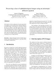
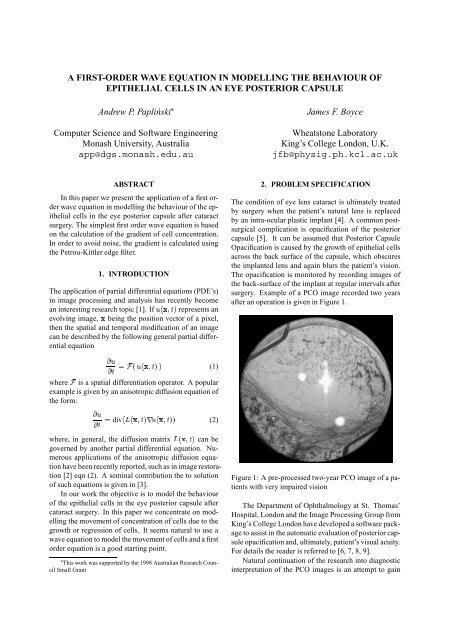
The opacification is monitored by record<strong>in</strong>g images <strong>of</strong><br />
<strong>the</strong> back-surface <strong>of</strong> <strong>the</strong> implant at regular <strong>in</strong>tervals after<br />
surgery. Example <strong>of</strong> a PCO image recorded two years<br />
after an operation is given <strong>in</strong> Figure 1.<br />
where, <strong>in</strong> general, <strong>the</strong> diffusion matrixL(x;t)can be<br />
governed by ano<strong>the</strong>r partial differential <strong>equation</strong>. Numerous<br />
applications <strong>of</strong> <strong>the</strong> anisotropic diffusion <strong>equation</strong><br />
have been recently reported, such as <strong>in</strong> image restoration<br />
[2] eqn (2). A sem<strong>in</strong>al contribution <strong>the</strong> to solution<br />
<strong>of</strong> such <strong>equation</strong>s is given <strong>in</strong> [3].<br />
In our work <strong>the</strong> objective is to model <strong>the</strong> <strong>behaviour</strong><br />
<strong>of</strong> <strong>the</strong> epi<strong>the</strong>lial cells <strong>in</strong> <strong>the</strong> eye posterior capsule after<br />
cataract surgery. In this paper we concentrate on modell<strong>in</strong>g<br />
<strong>the</strong> movement <strong>of</strong> concentration <strong>of</strong> cells due to <strong>the</strong><br />
growth or regression <strong>of</strong> cells. It seems natural to use a<br />
<strong>wave</strong> <strong>equation</strong> to model <strong>the</strong> movement <strong>of</strong> cells and a <strong>first</strong><br />
<strong>order</strong> <strong>equation</strong> is a good start<strong>in</strong>g po<strong>in</strong>t.<br />
This work was supported by <strong>the</strong> 1998 Australian Research Council<br />
Small Grant<br />
Figure 1: A pre-processed two-year PCO image <strong>of</strong> a patients<br />
with very impaired vision<br />
The Department <strong>of</strong> Ophthalmology at St. Thomas’<br />
Hospital, London and <strong>the</strong> Image Process<strong>in</strong>g Group from<br />
K<strong>in</strong>g’s College London have developed a s<strong>of</strong>tware package<br />
to assist <strong>in</strong> <strong>the</strong> automatic evaluation <strong>of</strong> posterior capsule<br />
opacification and, ultimately, patient’s visual acuity.<br />
For details <strong>the</strong> reader is referred to [6, 7, 8, 9].<br />
Natural cont<strong>in</strong>uation <strong>of</strong> <strong>the</strong> research <strong>in</strong>to diagnostic<br />
<strong>in</strong>terpretation <strong>of</strong> <strong>the</strong> PCO images is an attempt to ga<strong>in</strong>
understand<strong>in</strong>g and build ma<strong>the</strong>matical models <strong>of</strong> <strong>the</strong> underly<strong>in</strong>g<br />
recognized biological phenomena, namely, <strong>the</strong><br />
<strong>behaviour</strong> <strong>of</strong> <strong>the</strong> epi<strong>the</strong>lial cells on <strong>the</strong> surface <strong>of</strong> <strong>the</strong><br />
posterior capsule which obscures <strong>the</strong> back surface <strong>of</strong> <strong>the</strong><br />
implanted lens.<br />
In our work we will assume that <strong>in</strong>tensity <strong>of</strong> <strong>the</strong> PCO<br />
images is a measure <strong>of</strong> concentration <strong>the</strong> <strong>of</strong> epi<strong>the</strong>lial<br />
cells.<br />
@u @t=cgd(x;t)<br />
3. THE FIRST-ORDER WAVE EQUATION AND<br />
ITS COMPUTER MODELLING<br />
A simple <strong>first</strong> <strong>order</strong> <strong>wave</strong> <strong>equation</strong>, which describes movement<br />
<strong>in</strong> <strong>the</strong> directiondcan be written <strong>in</strong> <strong>the</strong> follow<strong>in</strong>g<br />
form:<br />
(3)<br />
gd(x;t)=dTru(x;t) (4)<br />
u(x;t+1)=u(x;t)+ctsjjru(x;t)jj<br />
experimentation we usen=4,l=3and=0:3. The<br />
(8)<br />
result<strong>in</strong>g discretised <strong>wave</strong> <strong>equation</strong> (7) takes <strong>the</strong> follow<strong>in</strong>g<br />
form:<br />
whereris a filtered gradient operation as described<br />
above. Note also <strong>the</strong> change <strong>of</strong> sign <strong>in</strong> <strong>order</strong> to be consistent<br />
with <strong>the</strong> usual notation <strong>in</strong> our class <strong>of</strong> images.<br />
In Figure 2 we demonstrate <strong>the</strong> <strong>behaviour</strong> <strong>of</strong> <strong>the</strong> <strong>wave</strong><br />
<strong>equation</strong> (8) <strong>in</strong> a one-dimensional case.<br />
1<br />
0.8<br />
0.6<br />
0.4<br />
<strong>in</strong>tensity<br />
u=u(dTxct)<br />
@u @t=cdu dv;ru=ddu<br />
andcis <strong>the</strong> speed <strong>of</strong> <strong>wave</strong> propagation. In <strong>order</strong> to show<br />
that<br />
(5)<br />
is a solution <strong>of</strong> eqn (3), we differentiate (3) with respect<br />
to time and space to obta<strong>in</strong><br />
gd=gTg<br />
from which <strong>the</strong> result follows immediately.<br />
In this paper we concentrated on modell<strong>in</strong>g <strong>the</strong> movement<br />
<strong>of</strong> <strong>the</strong> cell concentration <strong>in</strong> <strong>the</strong> direction <strong>of</strong> <strong>the</strong> concentration<br />
gradient.<br />
@u jjgjj=jjgjj<br />
@t=cjjg(x;t)jj<br />
In this case <strong>the</strong> projection <strong>of</strong> <strong>the</strong><br />
gradient on <strong>the</strong> direction <strong>of</strong> movement can be expressed<br />
as:<br />
(6)<br />
and <strong>the</strong> modell<strong>in</strong>g <strong>equation</strong> becomes<br />
(7)<br />
wherejjgjjis <strong>the</strong> gradient magnitude.<br />
In <strong>order</strong> to perform computer modell<strong>in</strong>g, eqn (7) needs<br />
to be discretised <strong>in</strong> <strong>the</strong> temporal and spatial doma<strong>in</strong>s.<br />
The time derivative is approximated by a simple backward<br />
time difference. As far as <strong>the</strong> gradient is concerned,<br />
it is important for real life images to calculate<br />
it us<strong>in</strong>g an appropriate low-pass filter. Most suitable<br />
for <strong>the</strong> purpose is an edge filter from <strong>the</strong> class <strong>of</strong> filters<br />
commonly referred to as Canny operators [10]. For<br />
our images, with very s<strong>of</strong>t edges we use a Petrou-Kittler<br />
edge filter [11] as described <strong>in</strong> [7] which is optimised<br />
for ramp edges. Such an edge operator is characterised<br />
by three parameters, namely, a number <strong>of</strong> filter<strong>in</strong>g directions,n,<br />
radial span,l, and angular overlap,. In our<br />
1.2<br />
1<br />
0.8<br />
0.6<br />
0.4<br />
0.2<br />
0<br />
0 10 20 30 40 50 60<br />
Figure 2: One-dimensional <strong>wave</strong> <strong>equation</strong><br />
The <strong>in</strong>itial distribution,u(x;0)and its gradientg(x;0)<br />
is marked with ’o’. Note that <strong>the</strong> fronts <strong>of</strong> <strong>the</strong> functions<br />
move accord<strong>in</strong>g to <strong>the</strong> value <strong>of</strong> gradient.<br />
For <strong>the</strong> real two-dimensional case results are presented<br />
<strong>in</strong> Figure 3. Images were down-sampled by <strong>the</strong><br />
factor <strong>of</strong> five, <strong>in</strong> <strong>order</strong> to reduce <strong>the</strong> size <strong>of</strong> <strong>the</strong> relevant<br />
postscript files.<br />
The <strong>first</strong> image represents <strong>the</strong> <strong>in</strong>itial concentration<br />
<strong>of</strong> cells. The boundary conditions are set so that <strong>the</strong><br />
cell concentration outside <strong>the</strong> lens’ disk is kept constant,<br />
namely,u=1, which is represented by <strong>the</strong> black colour<br />
<strong>in</strong> <strong>the</strong> images <strong>of</strong> Figure 3. With reference to eqns (7)and<br />
(8)<strong>the</strong> essential <strong>behaviour</strong> <strong>of</strong> <strong>the</strong> algorithms can be described<br />
as follows. Consider a ridge <strong>of</strong> cell concentration.<br />
The gradient <strong>of</strong> <strong>the</strong> top part <strong>of</strong> <strong>the</strong> ridge is zero<br />
which makes <strong>the</strong> position <strong>of</strong> <strong>the</strong> ridge is ma<strong>in</strong>ta<strong>in</strong>ed constant.<br />
For <strong>the</strong> slopes <strong>of</strong> <strong>the</strong> ridge, <strong>the</strong> magnitude <strong>of</strong> gradient<br />
is non-zero, which results <strong>in</strong> <strong>the</strong> slopes be<strong>in</strong>g flatten<br />
by mov<strong>in</strong>g <strong>the</strong>m apart. This elementary <strong>behaviour</strong> is<br />
comb<strong>in</strong>ed for each mound <strong>of</strong> cells to result <strong>in</strong> <strong>the</strong> emerg<strong>in</strong>g<br />
<strong>behaviour</strong> as observed <strong>in</strong> Figure 3. The islands <strong>of</strong><br />
cells are separated by flat grooves where gradient is zero<br />
or very small.<br />
It must be emphasized, however, that eqn (7) does<br />
not explicitly describe <strong>the</strong> growth or regression <strong>of</strong> cells,<br />
hence, <strong>the</strong> obta<strong>in</strong>ed patterns are poorer than that observed<br />
<strong>in</strong> <strong>the</strong> natural images.<br />
dressed <strong>in</strong> our future works.<br />
This issue will be ad-<br />
0.2<br />
wheregd(x;t)is <strong>the</strong> projection <strong>of</strong> <strong>the</strong> gradient <strong>of</strong> cell<br />
concentrationg=ru<strong>in</strong> <strong>the</strong> directiond, namely,<br />
0<br />
0 10 20 30 40 50 60<br />
1.4<br />
magnitude <strong>of</strong> gradient
C16d5P filtered gradient update, k = 1<br />
C16d5P filtered gradient update, k = 3<br />
C16d5P filtered gradient update, k = 5<br />
20<br />
20<br />
20<br />
40<br />
40<br />
40<br />
60<br />
60<br />
60<br />
80<br />
80<br />
80<br />
100<br />
100<br />
100<br />
120<br />
120<br />
120<br />
140<br />
140<br />
140<br />
160<br />
160<br />
160<br />
180<br />
180<br />
180<br />
20 40 60 80 100 120 140 160 180<br />
C16d5P filtered gradient update, k = 7<br />
20 40 60 80 100 120 140 160 180<br />
C16d5P filtered gradient update, k = 9<br />
20 40 60 80 100 120 140 160 180<br />
C16d5P filtered gradient update, k = 11<br />
20<br />
20<br />
20<br />
40<br />
40<br />
40<br />
60<br />
60<br />
60<br />
80<br />
80<br />
80<br />
100<br />
100<br />
100<br />
120<br />
120<br />
120<br />
140<br />
140<br />
140<br />
160<br />
160<br />
160<br />
180<br />
180<br />
180<br />
20 40 60 80 100 120 140 160 180<br />
C16d5P filtered gradient update, k = 13<br />
20 40 60 80 100 120 140 160 180<br />
C16d5P filtered gradient update, k = 15<br />
20 40 60 80 100 120 140 160 180<br />
C16d5P filtered gradient update, k = 17<br />
20<br />
20<br />
20<br />
40<br />
40<br />
40<br />
60<br />
60<br />
60<br />
80<br />
80<br />
80<br />
100<br />
100<br />
100<br />
120<br />
120<br />
120<br />
140<br />
140<br />
140<br />
160<br />
160<br />
160<br />
180<br />
180<br />
180<br />
20 40 60 80 100 120 140 160 180<br />
C16d5P filtered gradient update, k = 19<br />
20 40 60 80 100 120 140 160 180<br />
C16d5P filtered gradient update, k = 21<br />
20 40 60 80 100 120 140 160 180<br />
C16d5P filtered gradient update, k = 23<br />
20<br />
20<br />
20<br />
40<br />
40<br />
40<br />
60<br />
60<br />
60<br />
80<br />
80<br />
80<br />
100<br />
100<br />
100<br />
120<br />
120<br />
120<br />
140<br />
140<br />
140<br />
160<br />
160<br />
160<br />
180<br />
180<br />
180<br />
20 40 60 80 100 120 140 160 180<br />
20 40 60 80 100 120 140 160 180<br />
20 40 60 80 100 120 140 160 180<br />
Figure 3: Modell<strong>in</strong>g results for a PCO image
4. CONCLUSION<br />
In this paper we have demonstrated how a <strong>first</strong> <strong>order</strong><br />
<strong>wave</strong> <strong>equation</strong> can be used to model some aspects <strong>of</strong><br />
<strong>the</strong> propagation <strong>of</strong> epi<strong>the</strong>lial cells <strong>in</strong> <strong>the</strong> posterior capsule,<br />
namely, <strong>the</strong> formation <strong>of</strong> relatively regular islands<br />
<strong>of</strong> cells which gradually cover <strong>the</strong> whole back surface <strong>of</strong><br />
<strong>the</strong> capsule.<br />
Acknowledgment<br />
The authors would like to express <strong>the</strong>ir gratitude to Mr<br />
D. J. Spalton from <strong>the</strong> Department <strong>of</strong> Ophthalmology<br />
<strong>of</strong> St Thomas’ Hospital for <strong>the</strong> specification <strong>of</strong> <strong>the</strong> problem,<br />
<strong>the</strong> provision <strong>of</strong> <strong>the</strong> image data and for many useful<br />
discussions.<br />
5. REFERENCES<br />
[1] V. Caselles, J.-M. Morel, G. Sapiro, and A. Tannenbaum,<br />
“Introduction to <strong>the</strong> special issue on partial<br />
differential <strong>equation</strong>s and geometry driven diffusion<br />
<strong>in</strong> image process<strong>in</strong>g,” IEEE Transactions<br />
on Image Process<strong>in</strong>g, vol. 7, pp. 269–273, March<br />
1998.<br />
[8] A. P. Papliński and J. F. Boyce, “Co-occurrence arrays<br />
and edge density <strong>in</strong> segmentation <strong>of</strong> a class<br />
<strong>of</strong> ophthalmological images,” <strong>in</strong> Proceed<strong>in</strong>gs <strong>of</strong><br />
<strong>the</strong> 4rd Conference on Digital Image Comput<strong>in</strong>g:<br />
Techniques and Applications, DICTA97, (Auckland,),<br />
pp. 521–528, December 1997.<br />
[9] A. P. Papliński and J. F. Boyce, “Tri-directional<br />
filter<strong>in</strong>g <strong>in</strong> process<strong>in</strong>g a class <strong>of</strong> ophthalmological<br />
images,” <strong>in</strong> Proceed<strong>in</strong>gs <strong>of</strong> <strong>the</strong> IEEE Region<br />
10 Annual Conference, TENCON’97, (Brisbane),<br />
pp. 687–690, December 1997.<br />
[10] F. van der Heijden, “Edge and l<strong>in</strong>e feature extraction<br />
based on covariance models,” IEEE Trans.<br />
PAMI, vol. 17, pp. 16–33, January 1995.<br />
[11] M. Petrou and J. Kittler, “Optimal edge detectors<br />
for ramp edges,” IEEE Transactions on Pattern<br />
Analysis and Mach<strong>in</strong>e Intelligence, vol. 13,<br />
pp. 483–491, May 1991.<br />
[2] G. H. Cottet and M. El Ayyadi, “A Voltera type<br />
model for image process<strong>in</strong>g,” IEEE Transactions<br />
on Image Process<strong>in</strong>g, vol. 7, pp. 292–303, March<br />
1998.<br />
[3] P. Perona and J. Malik, “Scale space and edge detection<br />
us<strong>in</strong>g anisotropic diffusion,” IEEE Transactions<br />
on Pattern Analysis and Mach<strong>in</strong>e Intelligence,<br />
vol. 12, pp. 629–630, 1990.<br />
[4] S. A. Barman, J. F. Boyce, D. J. Spalton, P. G.<br />
Ursell, and E. J. Hollick, “Measurement <strong>of</strong> posterior<br />
capsule opacification,” <strong>in</strong> Proceed<strong>in</strong>gs <strong>of</strong> <strong>the</strong><br />
Conference on Medical Image Understand<strong>in</strong>g and<br />
Analysis, MIUA97, July 1997. Oxford, U.K.<br />
[5] D. J. Spalton and P. G. Ursell, “Incidence <strong>of</strong> PCO<br />
with PMMA, Acrilic and Silicone IOLs: Two year<br />
follow-up,” <strong>in</strong> Symposium on Cataract, IOL and<br />
Refractive Surgery. Congress on Ophthalmic Practice<br />
Management, June 1996. Seattle, Wash<strong>in</strong>gton.<br />
[6] A. P. Papliński and J. F. Boyce, “Segmentation<br />
<strong>of</strong> a class <strong>of</strong> ophthalmological images us<strong>in</strong>g a directional<br />
variance operator and co-occurrence arrays,”<br />
Optical Eng<strong>in</strong>eer<strong>in</strong>g, vol. 36, pp. 3140–<br />
3147, November 1997.<br />
[7] A. P. Papliński, “Directional filter<strong>in</strong>g <strong>in</strong> edge detection,”<br />
IEEE Trans. Image Proc., vol. 7, pp. 611–<br />
615, April 1998.