Using Quaternions for Parametrizing 3-D Rotations in ...

Jochen Schmidt and Heinrich Niemann
Using Quaternions for Parametrizing 3–D Rotations in Unconstrained Nonlinear Optimization
appeared in:
Vision, Modeling, and Visualization 2001 (VMV 2001)
Stuttgart, Germany
p. 399-406
666

Using Quaternions for Parametrizing 3–D Rotations in Unconstrained
Nonlinear Optimization
J. Schmidt and H. Niemann
Chair for Pattern Recognition (Informatik 5), University of Erlangen–Nuremberg
Martensstr. 3, 91058 Erlangen, Germany
Email: {jschmidt,niemann}@informatik.uni-erlangen.de
Abstract
In this paper we address the problem of using
quaternions in unconstrained nonlinear optimization
of 3-D rotations. Quaternions representing rotations
have four elements but only three degrees
of freedom, since they must be of norm one. This
constraint has to be taken into account when applying
e. g. the Levenberg-Marquardt algorithm, a
method for unconstrained nonlinear optimization
widely used in computer vision. We propose an
easy to use method for achieving this. Experiments
using our parametrization in photogrammetric
bundle-adjustment are presented at the end of the
paper.
1 Introduction
Many tasks in computer vision require the estimation
of 3-D rotation matrices, usually using a linear
algorithm first and a nonlinear refinement afterwards.
Examples include camera calibration [2, 3]
or photogrammetric bundle-adjustment [4, 6, 10,
3] in structure-from-motion applications. An often
used [4, 6, 10, 3] method for doing nonlinear
refinement is the Gauss-Newton algorithm with
Levenberg-Marquardt extension [3, 11], which is an
iterative algorithm for unconstrained optimization.
Since a 3×3 rotation matrix has 9 elements but only
3 degrees of freedom (DOF), other parametrizations
are used for rotations in 3-D: Euler angles,
axis/angle representation, and quaternions.
Quaternions have advantages in many applications,
they are used for example in computer vision
for a numerically stable estimation of rotation from
an essential matrix [2], or in computer graphics for
interpolation between two given rotations, since the
use of quaternions yields smooth movements, while
Euler angles do not [16].
This contribution focuses on quaternions, but
because of the strong dependencies between
axis/angle representation and quaternions a short review
of the other two parametrizations is given first.
2 Parametrizing Rotations
2.1 Fair Parametrizations
The term fair parametrization was introduced by
Hornegger and Tomasi in [8]. A parametrization
is called fair, if it does not introduce more numerical
sensitivity than inherent to the problem itself.
This is guaranteed, if any rigid transformation of
the space to be parametrized results in an orthogonal
transformation of the parameters. Since this
is a rather general definition, it is not restricted to
parametrizing rotations, but in [8] the parametrization
of camera motion is treated.
2.2 Euler Angles
Representing a rotation by Euler angles is probably
the best known parametrization. A rotation matrix
can be built from three matrices representing
rotations around the axes of the coordinate-system,
where each rotation is defined by an angle. As
matrix multiplication is not commutative, the Euler
angle representation is not unique, meaning that
a permutation of the order of the rotations around
the axes yields different Euler angles. Probably the
most important drawback of this parametrization is
the existence of so-called gimbal lock singularities,
where one DOF is lost, i. e. two of the three Euler
angles belong to the same DOF. For a deeper discussion
see [16].
Since Euler angles are not a fair parametrization
of rotations according to [8] either and thus are nu-
VMV 2001 Stuttgart, Germany, November 21–23, 2001

θ
axis a
quaternions in computer vision can be found in [2].
They are a fair parametrization in the sense of [8].
A quaternion h is defined as follows:
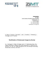
Figure 1: Rotation around an axis a by angle θ.
merically instable for estimating rotations, we do
not discuss them any further.
2.3 Axis/Angle Representation
The parametrization most widely used in bundleadjustment
[6, 7, 13] is the axis/angle representation.
It is a fair parametrization in the sense of [8].
=
An arbitrary rotation R ∈ IR 3×3 can be represented
as a rotation around one axis a ∈ IR 3 by the
angle θ (see Figure 1). Since only the direction of
the rotation axis a is of importance, a has only 2
DOF. Hence axis and angle can be combined into a
single 3-vector, its direction giving the rotation
axis and its length the rotation angle:
θ = ||, a . (1)
||
Computing a rotation matrix R fromcan be done
by using the formula of Rodrigues [2]:
R = e [] ×
= I sin θ 3+
θ [] 1 − cos θ
×+ [] 2 θ 2 × ,
(2)
where [] × is the following antisymmetric matrix:
=¾¼ω =¼0 −ω 3 ω 2
[] × ω 3 0 −ω 1
1
ω 2
ω 3½¿×
(3)
The computation of axis and angle from a rotation
matrix R can be done as follows [15]: Eigendecomposition
of R yields the three Eigen-values 1
and cos θ ± isin θ. The axis a is the Eigen-vector
corresponding to the Eigen-value 1. The angle θ can
now be calculated from one of the remaining Eigenvalues.
The consistency of the direction of the axis
and the angle can be checked by inserting them into
equation (2).
2.4 Quaternions
−ω 2 ω 1 0½.
Quaternions are numbers, in a certain sense similar
to complex numbers: Instead of using only
one imaginary part, three are introduced. More on
h = w+xi+yj+zk, w, x,y, z ∈ IR , (4)
where w is the real part and x,y, z are the imaginary
parts. Multiplication and summation are done
component-wise, with
i 2 = j 2 = k 2 = −1 ,
ij = −ji = k ,
jk = −kj = i ,
ki = −ik = j .
(5)
Often a quaternion is written as a 4-tupel h =
(w, x, y, z) or h = (w,v), where v is a 3-vector
containing the imaginary parts. In contrast to complex
numbers, the commutative law of multiplication
is not valid, i. e. h 1h 2 ≠ h 2h 1. Similar to
complex numbers, a conjugate quaternion is defined
as h = w −xi −yj −zk. The norm of a quaternion
h is |h| =Ôh · h =Ôw 2 + x 2 + y 2 + z 2 . For
unit quaternions (|h| = 1), the inverse of multiplication
equals the conjugate: h −1 = h.
Just as the multiplication of two unit complex
numbers defines a rotation in 2-D, a multiplication
of two unit quaternions yields a rotation in 3-D. Let
p be a 3-D point to be rotated, a a rotation axis
with |a| = 1, and θ the angle of rotation around
this axis as in Section 2.3. Define the following two
quaternions:
h =cos θ 2 ,sin θ 2 · a,
(6)
p ′ = (0,p) .
a¡
Then
p ′ rot = h · p′ · h , (7)
where p ′ rot is the quaternion corresponding to the
rotated point.
Note that the representation of a rotation as a
quaternion (and also as axis/angle) is not unique,
since the two quaternions h 1 = cos θ ,sin θ · 2 2
and h 2 = −cos θ , − sin θ · a¡define the same
2 2
rotation. This is a direct result of the axis/angle representation,
because a rotation around an axis a by
an angle θ is the same as a rotation around the axis
−a by the angle 2π − θ. Which one of the two
quaternions is used does not matter, but one has to
666

e careful when measuring the distance of two rotations
(e. g. for describing the calibration error) by
the distance between quaternions.
The computation of a quaternion from a rotation
matrix is done using the axis/angle representation
as described in equation (6). The computation of a
rotation matrix R from a quaternion can be done as
follows [2]:
where
r 1 =¼h
R = r 1 r 2 r 3¡, (8)
2
0 + h 2 1 − h 2 2 − h 2 3
2(h 1h 2 + h 0h 3)
2)½,
2(h 1h 3 − h 0h
1)½,
2(h 2h 3 + h 0h
3½.
h 2 0 − h 2 1 − h 2 2 + h 2
r 2 =¼2(h 1h 2 − h 0h 3)
h 2 0 − h 2 1 + h 2 2 − h 2 3
r 3 =¼2(h 1h 3 + h 0h 2)
2(h 2h 3 − h 0h 1)
(9)
3 Unconstrained Nonlinear Optimization
Nonlinear Optimization is usually performed after
a linear step, i. e. an initial estimation of the rotation
matrix exists already. The corresponding
quaternion is denoted here as h 0. When using an
unconstrained nonlinear optimization method like
the Levenberg-Marquardt algorithm, the main problem
is that a quaternion representing a rotation
has four elements but only 3 DOF because of the
norm–1 constraint. This has to be considered during
the optimization process. Additionally a minimal
parametrization is desired because of computation
time, especially if we consider the problem
of bundle-adjustment where many 3-D rotations are
optimized simultaneously.
3.1 Possible Solutions
At the beginning of this section we will discuss
some possible solutions for this problem, after that
our approach is described in detail.
Use all four elements of the quaternion. The
simplest way to do nonlinear optimization using
quaternions is to ignore the norm–1 constraint completely
and change all four elements. After optimization,
the resulting quaternion is forced to
norm 1. This approach has two drawbacks: On the
one hand, four parameters are changed where three
would be sufficient, on the other hand the norm
changes during optimization, while it would be desired
to be preserved.
Lagrange. A standard way to deal with constraints
is the introduction of Lagrangian multipliers.
Therefore the function to be optimized must
be extended by a term of the form λ i(h T i h i − 1).
This is not a problem in principle, but has the disadvantage
that the number of parameters to be estimated
increases from four to five, because of the
Lagrangian multipliers λ i. In bundle-adjustment,
where a whole image sequence is processed at once
and thus a rotation has to be computed for each
image, this results in additional computation time
needed.
One possibility would be to fix the λ i before optimization
in order regularize the problem instead of
estimating them. This approach punishes deviations
from the norm–1 constraint by increasing the residual.
An exact compliance (within numerical precision)
with the constraint however is not ensured,
and additionally the question arises to what values
to fix the λ i.
Use only the imaginary parts of the quaternion.
This parametrization is used in [1], but not for nonlinear
optimization. Three parameters κ x, κ y, and
κ z are changed here, from which the quaternion h
is calculated as
h =Ö1 − (κ2 x + κ 2 y + κ 2 z)
, κx
4 2 , κy
2 , κz
2.
(10)
The advantage is that only the minimum number of
three parameters is used. But it has to be made sure
that the changes are done in a way that the radicand
is always positive, which cannot be guaranteed
when performing Levenberg-Marquardt optimization.
This is why we do not use this approach.
Conclusion: A parametrization has to be found,
that:
• is minimal, i. e. it uses only three parameters,
666

h 0
v
θ
O
h v
h Z
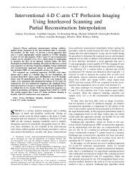
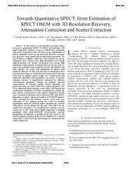
Figure 2: Parametrization of rotation by quaternions:
The tangential hyperplane touches the unit
sphereË3 in h 0. h v is the quaternion lying in this
hyperplane, h Z is the resulting quaternion.
• the three parameters can be changed arbitrarily
by the optimization algorithm,
• the resulting quaternion has always norm 1.
In the following we present a technique for accomplishing
this.
3.2 New Approach
We now describe a way for parametrizing changes
in rotation starting at an initial solution obtained
e. g. by a linear method. We will call that starting
quaternion h 0 the operating point. All quaternions
of norm 1 lie on the unit sphere in IR 4 , i. e. theË3 .
The goal is to use three parameters for giving the direction
and distance of the resulting quaternion on
this sphere. Therefore we use the shortest connection
between two points on a sphere, i. e. a great circle.
In the following we will show how this can be
accomplished. Figure 2 shows the general setting.
For describing a movement on the sphere starting
at h 0 we use a vector v 4 ∈ IR 4 lying in the
tangential hyperplane that touches the sphere in h 0.
This hyperplane is a subspace of IR 4 , thus vectors
in this plane can be represented as 3-vectors with
respect to a local coordinate system spanning the
plane. The corresponding 3-vector to v 4 we call
v ∈ IR 3 . The origin of this system is h 0.
Therefore we use a 3-vector encoding a direction
along a great circle, its length giving the distance
to move on the great circle for parametrizing
quaternions in nonlinear optimization. Since we
consider quaternions lying on a unit sphere, the distance
equals the angle between the operating point
h 0 and the resulting quaternion h Z measured in radian.
The great circle on which the movement is to
be done is defined by intersecting the sphere with
the 2-D plane through the origin that is spanned by
the operating point h 0 and v 4. The further text is
divided in three parts:
1. Computation of an orthogonal basis of the tangential
hyperplane. This basis is the local coordinate
system for v.
2. Conversion of the 3-vector v to a 4-vector lying
in the hyperplane.
3. Computation of the resulting quaternion h Z.
3.2.1 Basis of the Tangential Hyperplane
First we compute the hyperplane tangential to the
sphere in h 0. This plane is defined by all points
x ∈ IR 4 satisfying
h 0 T x = 1 , (11)
since h 0 is a normal vector of the plane. In order to
distinguish the normal vector from the quaternion,
in the following we denote the normal vector by n.
But one should keep in mind that
n = n 1 n 2 n 3 n 4¡T
= h0 . (12)
This gives the plane equation in normal form:
n 1x 1 + n 2x 2 + n 3x 3 + n 4x 4 − 1 = 0 . (13)
Since we do not need this equation but rather a basis
of the subspace defined by this plane, we convert
equation (13) to parameter form. Therefore we
choose one element of n not equal to zero 1 . Let
this be without loss of generality n 1. Now choose
the three parameters λ = x 2, µ = x 3 and ν = x 4.
Plugging these into (13) and solving for x 1 gives:
x 1 = 1 n 1
(1 − n 2x 2 − n 3x 3 − n 4x 4) ,
x 2 = λ, x 3 = µ, x 4 = ν .
Thus we get a parameter form of the plane:
(14)
x = a + λb ′ 1 + µb ′ 2 + νb ′ 3 , (15)
1 there will always be one n i not equal to zero, since |n| = 1.
666

where
a =
1
n 1
0 0 0¡T
,
b ′ 1 = − n 2
n 1
1 0 0¡T
,
(16)
b ′ 2 = − n 3
n 1
0 1 0¡T
,
b ′ 3 = − n 4
n 1
0 0 1¡T
.
Now we have a basis B ′ for the hyperplane:
B ′ = b ′ 1 b ′ 2 b ′ 3¡. (17)
Note that this basis is not yet orthogonal. To avoid
numerical instabilities an orthogonal basis B is
computed from B ′ . Therefore we use the singular
value decomposition (SVD) [11] of B ′ which is
given as:
B ′ = BΣV T . (18)
Then the 4 × 3 matrix B is an orthonormal basis
spanning the same subspace as B ′ .
3.2.2 3-D/4-D Conversion of v
Given an arbitrary 3-vector v with respect to the
basis B, a 4-vector v 4 lying in the tangential hyperplane
can be computed by:
v 4 = Bv . (19)
3.2.3 Computing the Resulting Quaternion
The quaternion h Z we look for lies on the great circle
defined by the intersection of the sphere with the
2-D plane through the origin spanned by h 0 and v 4:
x = λh 0 + µv 4N , (20)
where
v 4N = v4
. (21)
|v 4|
Normalization of v 4 is of course not necessary for
establishing the plane equation (20). The following
computations will become more clear, however.
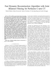
The vectors h 0 and v 4N build an orthogonal coordinate
system whose origin coincides with the origin
of the sphere. The quaternion h Z is a vector lying in
that plane building an angle θ with h 0 (see Figure
3). We get h Z as a linear combination of the two
vectors spanning the plane:
where
h Z = sin(θ)v 4N + cos(θ)h 0 , (22)
θ = |v 4| . (23)
It is easily shown that the resulting quaternion h Z is
of norm 1.
h 0
θ
sin θ
h Z
v 4N
cos θ
Figure 3: The vectors h 0 and v 4N give an orthonormal
basis of the plane containing the resulting
quaternion h Z .
3.2.4 Summary
We will now give a short summary of the steps necessary
to use our parametrization. Before performing
the nonlinear optimization do once:
• compute operating point h 0 from given rotation
matrix,
• compute basis vectors b ′ i (i = 1, 2, 3), build a
4 × 3 matrix B ′ ,
• compute an orthonormal basis B from B ′ using
SVD,
• initialize parameter vector v = 0 .
During optimization only the following computations
are necessary to get an optimized quaternion
h Z from the parameter vector v:
• convert the 3-vector v to a 4-vector v 4 using
equation (19),
• compute the resulting quaternion h Z from v 4
using equation (22),
• if desired convert h Z to a rotation matrix using
equation (8).
4 Experimental Results
For the experiments we chose photogrammetric
bundle-adjustment [4, 6, 10, 3], i. e. nonlinear optimization
of camera parameters and scene points
using multiple views of a scene simultaneously.
Bundle-adjustment minimizes the back-projection
error, i. e. the root mean square error per image
666

ÚÙØ1
mn
point in pixels, which is given by:
mi=1
(x ij − ˜x ij) 2 + (y ij − ỹ ij) 2¡,
nj=1
500
(24)
where n is the number of frames, m the number of
3-D points, (x ij, y ij) a detected feature point, and
(˜x ij, ỹ ij) the back-projection of a reconstructed
3-D point i into frame j.
Before bundle-adjustment, a linear structurefrom-motion
method was applied to get an initial
reconstruction of scene geometry and camera positions.
This method is described in [5]; it is based
upon [14], and by applying self-calibration methods
[3] reconstruction is possible up to an unknown
similarity transformation. Since the camera matrices
obtained this way are still slightly projectively
distorted, they are forced to be Euclidean by orthogonalization
of rotation matrices using SVD.
For bundle-adjustment we applied our own implementation
of the Levenberg-Marquardt algorithm,
which is capable of exploiting the special
block-structure of the Jacobian in interleaved
bundle-adjustment [13]. More details on the algorithm
and the experiments can be found in [12].
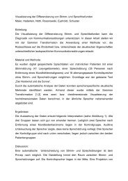
We used 8 scenes generated synthetically,
i. e. with known ground truth, two of which are
shown in Figure 4. First we give a short summary
of their properties:
• Each scene consists of 100 3-D points in 20
frames. The points were randomly distributed
within a cube of side length 200 mm. Each
point is visible in all frames.
• The distance and viewing direction of each
camera was varied randomly, thus simulating
the behaviour of a hand-held camera.
• The focal lengths f x and f y were chosen randomly
from the intervall 800 – 1200 pixels,
assuming quadratic pixels, i. e. f x = f y. The
values for f x and f y were chosen such that they
correspond to a camera with a 1/2”-CCD-Chip
and a focal length of 8 mm. Therefore the coordinates
of the image points are of the same
order of magnitude as in a PAL-image.
• The principal point (u 0, v 0) was chosen as
(0, 0).
• The 3-D points were projected into each
frame, Gaussian noise with standard deviation
σ of 0.3, 0.7, and 1.0 pixel was added independently
for each coordinate, giving a total
400
300
200
100
0
−100
−200
−300
−400
−500
0
50
50
0
−50
0
−50
0
100
200
300
(a) radial camera motion
−400
−300
−200
−100
0
100
200
400
300
(b) translatorial camera motion
Figure 4: Examples of the scenes used for simulation:
The 3-D world points (circles) are located
within a cube centered at the origin, the camera was
moved in a radial (a) or translatorial (b) way. The
arrows give the viewing direction of the cameras at
their respective position. All units in mm.
of 24 different image sequences.
In Table 1 we give some selected results from our 24
sequences obtained after 20 Levenberg-Marquardt
iterations; the complete results are contained in
[12].
The back-projection error is given before and after
nonlinear optimization. The two values before
optimization correspond to the error before (left
value) and after (right value) orthogonalizing the
rotation matrix, since this results in an increasing
back-projection error. For the camera parameters
we give the root mean square error before optimization
and the change in error of the parameter with
respect to the value before optimization. Thus one
400
500
500
666

Table 1: Back-projection error before (bef.) and after optimization, changes in error in camera parameters
using quaternions (Quat.) and axis/angle representation (A/A). In scenes 1-4 camera motion was radial, in
scenes 5-8 translatorial. Gaussian noise with different standard deviations σ was added to the image points.
Scene σ f x f y u 0 v 0 t R 3-D Back-proj. Error
bef. 8.60 8.13 9.96 4.37 2.21369 0.00269973 0.243482 0.45/0.49
1 0.3 Quat. -4.09 -3.28 -7.69 -2.74 -0.882988 -0.00201266 -0.14373 0.40
A/A -4.10 -3.28 -7.65 -2.75 -0.885005 -0.00200837 -0.14363 0.40
bef. 36.0 36.5 38.9 26.1 9.57001 0.0110419 0.984122 1.50/1.86
2 1.0 Quat. -7.89 -8.12 -21.8 -15.2 -1.97096 -0.00637703 -0.504492 1.31
A/A -7.86 -7.83 -19.2 -15.0 -1.97941 -0.00573987 -0.490924 1.32
bef. 32.9 32.8 22.7 20.8 9.44783 0.00895585 1.99887 1.74/1.86
3 1.0 Quat. -27.2 -27.0 -15.5 -12.7 -6.37081 -0.00612914 -1.04459 1.33
A/A -27.2 -27.1 -15.5 -12.6 -6.39037 -0.00610905 -1.06381 1.33
bef. 88.7 91.4 47.5 41.1 26.6822 0.0138212 1.78132 1.20/1.73
4 0.7 Quat. -12.4 -15.4 -12.6 -13.5 -3.73035 -0.00545732 -0.81368 0.98
A/A -14.0 -17.3 -19.4 -16.6 -4.64984 -0.00657011 -0.967142 0.96
bef. 45.1 47.2 18.7 13.9 30.3697 0.00762509 8.95917 1.53/2.08
5 1.0 Quat. 2.21 0.765 -4.29 -4.46 -4.61299 -0.0026916 -2.61643 1.31
A/A 3.27 1.61 -4.99 -4.07 -4.45546 -0.00257544 -2.65749 1.31
bef. 340 346 171 128 91.9583 0.0623885 8.46183 1.86/3.95
6 1.0 Quat. -1.68 -8.46 -0.940 -1.50 0.173968 0.00652012 -0.397551 1.70
A/A -2.52 -9.48 0.281 -1.50 0.0102833 0.00716027 -0.254497 1.70
bef. 14.7 15.5 12.7 9.67 4.98782 0.00387035 0.320034 0.45/0.48
7 0.3 Quat. -3.27 -4.05 -7.08 -4.73 -1.13315 -0.00201028 -0.145408 0.39
A/A -3.23 -4.01 -6.95 -4.66 -1.11664 -0.00197918 -0.144794 0.39
bef. 27.7 27.0 28.6 19.7 9.38349 0.00846833 0.667536 1.01/1.11
8 0.7 Quat. -16.7 -16.1 -20.2 -11.3 -6.00133 -0.00561137 -0.35916 0.91
A/A -17.0 -16.5 -21.5 -12.7 -6.13845 -0.00602556 -0.361227 0.91
can see immediately how large the change was, and,
by looking at the sign, whether the error became
larger (+) or smaller (−) during optimization. For
measuring the error in rotations (R) we use the Euclidean
distance between two quaternions. In the
table, the root mean square error per component of
the quaternion is given. For translation (t) the Euclidean
distance between two translation vectors is
used similar to rotation, i. e. the table gives the error
per component of the vector. The 3-D error denotes
the root mean square error (and its change)
per world point. In Table 2 the change in error in
rotation is given in percent.
To summarize the results we obtained: It is
not possible to tell in general which of the two
parametrizations to prefer for bundle-adjustment.
The decrease in error in focal length, principal
point, translation, and 3-D points was larger when
using quaternions instead of axis/angle representation
in about 50% of our experiments, and vice
versa. If we look at the change in error for rotation
only, we get better results for quaternions than
for axis/angle representation in about 70.8% of the
experiments, the difference in change of error between
quaternions and axis/angle ranging from be-
Table 2: Changes in error in rotation in percent for
the data given in Table 1 with respect to the error
after the linear algorithm and orthogonalization of
the rotation matrix.
Scene σ Quat. A/A
1 0.3 -74.55% -74.39%
2 1.0 -57.75% -51.98%
3 1.0 -68.44% -68.21%
4 0.7 -39.49% -47.54%
5 1.0 -35.30% -33.78%
6 1.0 +10.45% +11.48%
7 0.3 -51.94% -51.14%
8 0.7 -66.26% -71.15%
low 1% to about 5% (see Table 2). With both representations
change in error is relatively high, in many
cases more than 50% with respect to the error after
the linear algorithm and orthogonalization. Thus
we can recommend our quaternion parametrization
if special focus is set on error in rotation, even if it
is not guaranteed to yield always better results than
axis/angle representation.
666

5 Conclusions
In this paper we presented an easy to use and accurate
method for applying the quaternion representation
of 3-D rotations in unconstrained nonlinear
optimization problems using e. g. the Levenberg-
Marquardt algorithm. In order to prove the practical
applicability of this parametrization, we used it in
photogrammetric bundle-adjustment for estimating
camera parameters as well as 3-D scene points starting
from an initial reconstruction obtained by a linear
factorization method. The experiments showed
that our parametrization should be used especially
when good estimations for rotations are needed.
References
[1] A. Azarbayejani and A. P. Pentland. Recursive
estimation of motion, structure, and focal
length. IEEE Trans. on Pattern Analysis and
Machine Intelligence, 17(6):562–575, 1995.
[2] Oliver Faugeras. Three-Dimensional Computer
Vision: A Geometric Viewpoint. MIT
Press, Cambridge, MA, 1993.
[3] R. Hartley and A. Zisserman. Multiple View
Geometry in computer vision. Cambridge
University Press, Cambridge, 2000.
[4] R. I. Hartley. Euclidean Reconstruction from
Uncalibrated Views, volume 825 of Lecture
notes in Computer Science, pages 237–256.
Springer-Verlag, 1994.
[5] B. Heigl and H. Niemann. Camera calibration
from extended image sequences for lightfield
reconstruction. In B. Girod, H. Niemann, and
H.-P. Seidel, editors, Vision Modeling and Visualization
99, pages 43–50, Erlangen, Germany,
Nov. 1999. Infix.
[6] A. Heyden and K. Åström. Euclidean reconstruction
from image sequences with varying
and unknown focal length and principal
point. In Proceedings of Computer Vision
and Pattern Recognition, pages 438–443,
Puerto Rico, Juni 1997. IEEE Computer Society
Press.
[7] A. Heyden and K. Åström. Flexible calibration:
Minimal cases for auto-calibration. In
ICCV 99 [9], pages 350–355.
[8] J. Hornegger and C. Tomasi. Representation
issues in the ML estimation of camera motion.
In ICCV 99 [9], pages 640–647.
[9] Proceedings of the 7 th International Conference
on Computer Vision (ICCV), Corfu,
September 1999. IEEE Computer Society
Press.
[10] P. F. McLauchlan. Gauge invariance in projective
3D reconstruction. In Proceedings of
the IEEE Workshop on Multi-View Modeling
& Analysis of Visual Scenes, Fort Collins, Colorado,
June 1999.
[11] W. H. Press, S. A. Teukolsky, W. T. Vetterling,
and B. P. Flannery. Numerical Recipes in C:
The Art of Scientific Computing. Cambridge
University Press, 2nd edition, 1992.
[12] J. Schmidt. Erarbeitung geeigneter Optimierungskriterien
zur Berechnung von Kameraparametern
und Szenengeometrie aus Bildfolgen.
Diplomarbeit, Lehrstuhl für Mustererkennung,
Universität Erlangen-Nürnberg,
2000.
[13] H.-Y. Shum, Q. Ke, and Z. Zhang. Efficient
bundle adjustment with virtual key frames: A
hierarchical approach to multi-frame structure
from motion. In Proceedings of Computer Vision
and Pattern Recognition, volume 2, pages
538–543, Fort Collins, Colorado, Juni 1999.
IEEE Computer Society Press.
[14] P. Sturm and B. Triggs. A factorization based
algorithm for multi–image projective structure
from motion. In B. Buxton and R. Cipolla,
editors, Computer Vision — ECCV ’96, number
1065, pages 709–720, Heidelberg, 1996.
Springer.
[15] E. Trucco and A. Verri. Introductory Techniques
for 3–D Computer Vision. Prentice
Hall, New York, 1998.
[16] A. Watt and M. Watt. Advanced Animation
and Rendering Techniques. Addison-Wesley,
1992.
666