4 - People.stat.sfu.ca
4 - People.stat.sfu.ca
4 - People.stat.sfu.ca

You also want an ePaper? Increase the reach of your titles
YUMPU automatically turns print PDFs into web optimized ePapers that Google loves.
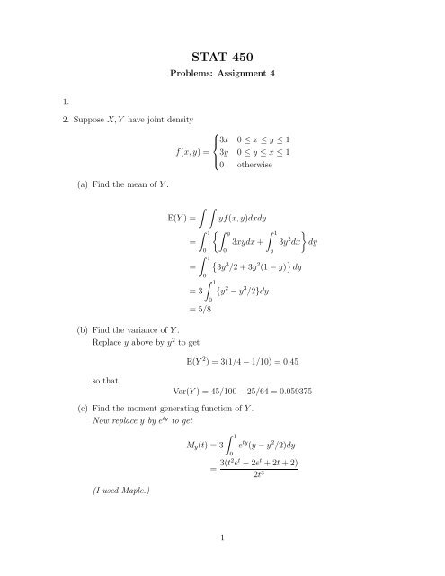
STAT 450<br />
Problems: Assignment 4<br />
1.<br />
2. Suppose X, Y have joint density<br />
⎧<br />
⎪⎨ 3x 0 ≤ x ≤ y ≤ 1<br />
f(x, y) = 3y 0 ≤ y ≤ x ≤ 1<br />
⎪⎩<br />
0 otherwise<br />
(a) Find the mean of Y .<br />
∫ ∫<br />
E(Y ) = yf(x, y)dxdy<br />
∫ 1<br />
{∫ y<br />
= 3xydx +<br />
=<br />
= 3<br />
0<br />
∫ 1<br />
0<br />
∫ 1<br />
0<br />
= 5/8<br />
(b) Find the variance of Y .<br />
Replace y above by y 2 to get<br />
0<br />
∫ 1<br />
y<br />
}<br />
3y 2 dx dy<br />
{<br />
3y 3 /2 + 3y 2 (1 − y) } dy<br />
{y 2 − y 3 /2}dy<br />
E(Y 2 ) = 3(1/4 − 1/10) = 0.45<br />
so that<br />
Var(Y ) = 45/100 − 25/64 = 0.059375<br />
(c) Find the moment generating function of Y .<br />
Now replace y by e ty to get<br />
∫ 1<br />
M y (t) = 3 e ty (y − y 2 /2)dy<br />
0<br />
= 3(t2 e t − 2e t + 2t + 2)<br />
2t 3<br />
(I used Maple.)<br />
1
3. Find the moment generating function of the number of tails before the first head when<br />
you toss a coin with probability p of landing heads.<br />
We have<br />
so that<br />
P (X = k) = p(1 − p) k k = 0, 1, · · ·<br />
M X (t) = p<br />
=<br />
∞∑ { } (1 − p)e<br />
t k<br />
0<br />
p<br />
1 − (1 − p) exp(t)<br />
4. Suppose X is a random variable with mean µ and variance σ 2 . Find the value of a<br />
which minimizes<br />
E{(X − a) 2 }.<br />
Define h(b) by<br />
h(a) = E [ (X − a) 2]<br />
= E [ (X 2 − 2aX + a 2 ) ]<br />
= E(X 2 ) − 2aE(X) + a 2<br />
To minimize h set<br />
h ′ (a) = 2a − 2E(X) = 0<br />
and solve to find a = E(X). That this is a minimum follows from h ′′ = 2 > 0 for all<br />
a.<br />
5. Find the mean and variance of the density<br />
{<br />
|1 − x| 0 ≤ x ≤ 2<br />
f(x) =<br />
0 otherwise<br />
E(X) =<br />
=<br />
∫ 2<br />
0<br />
∫ 1<br />
0<br />
xf X (x) dx<br />
x(1 − x) dx +<br />
∫ 2<br />
1<br />
x(x − 1) dx<br />
= ( x 2 /2 − x 3 /3 )∣ ∣ 1 0 + ( x 3 /3 − x 2 /2 )∣ ∣ 2 1<br />
= 1/6 + [(8/3 − 2) − (1/3 − 1/2)]<br />
= 1<br />
2
(which is to be expected be<strong>ca</strong>use the density is symmetric about x = 1.) Also:<br />
E(X 2 ) =<br />
=<br />
∫ 2<br />
0<br />
∫ 1<br />
0<br />
x 2 f X (x) dx<br />
x 2 (1 − x) dx +<br />
∫ 2<br />
1<br />
x 2 (x − 1) dx<br />
= ( x 3 /3 − x 4 /4) )∣ ∣ 1 0 + ( x 4 /4 − x 3 /3 )∣ ∣ 2 1<br />
= 1/(12) + [(16/4 − 8/3) − (1/4 − 1/3)]<br />
= 3/2<br />
Hence<br />
Var(X) = E(X 2 ) − [E(X)] 2 = 1/2 .<br />
6. Find the mean and variance of the Rayleigh density<br />
{<br />
λ 2 xe −λ2 x 2 /2<br />
x > 0<br />
f(x) =<br />
0 otherwise<br />
E(X r ) =<br />
=<br />
∫ ∞<br />
0<br />
∫ ∞<br />
0<br />
x r f X (x) dx<br />
x r λ 2 xe −(λx)2 /2 dx<br />
Make the substitution y = (λx) 2 /2 and dy = λ 2 xdx to see that<br />
E(X r ) =<br />
∫ ∞<br />
0<br />
(2y) r<br />
e −y dy<br />
λ r<br />
∫ ∞<br />
= 2 r/2 λ −r y r/2+1−1 e −y dy<br />
The integral matches the definition of the Gamma function precisely so<br />
In particular<br />
E(X r ) = 2r/2 Γ(1 + r/2)<br />
λ r<br />
E(X) = 2 1/2 Γ(3/2)/λ<br />
(In fact Γ(3/2) = (1/2)Γ(1/2) = π 1/2 /2 but I don’t really expect you to know this!)<br />
Moreover<br />
E(X 2 ) = 2Γ(2)/λ 2 = 2/λ 2<br />
and<br />
Var(X) = 2 λ 2 − ( 2 1/2 Γ(3/2)/λ ) 2<br />
= (2 − π/2)/λ<br />
2<br />
0<br />
3
7. Find the mean and variance of the Maxwell density<br />
{<br />
4λ 3 x 2 e −λ2 x 2 / √ π<br />
f(x) =<br />
0 otherwise<br />
E(X r ) =<br />
=<br />
∫ ∞<br />
0<br />
∫ ∞<br />
0<br />
x r f X (x) dx<br />
4x r λ 3 x 2 e −(λx)2 dx/ √ π<br />
Make the substitution y = (λx) 2 and dy = 2λ 2 xdx to see that<br />
E(X r ) =<br />
∫ ∞<br />
2y (r+1)/2<br />
0<br />
= 2<br />
λ r√ π<br />
λ r√ π e−y dy<br />
∫ ∞<br />
0<br />
= 2<br />
λ r√ Γ((r + 3)/2)<br />
π<br />
y (r+1)/2+1−1 e −y dy<br />
In particular<br />
and<br />
E(X) = 2<br />
λ √ π Γ(2) = 2<br />
λ √ π<br />
E(X 2 ) = 2<br />
λ 2√ π Γ(5/2) = 3<br />
2λ 2√ π Γ(1/2) = 3<br />
2λ 2<br />
Var(X) = (3/2 − 4/π)/lambda 2 .<br />
8. Suppose X and Y are random variables such that X is Uniform[0,1] and<br />
{<br />
1 x < y < x + 1<br />
f Y |X (y|x) =<br />
0 otherwise<br />
(a) Find E(Y ).<br />
4
∫ ∫<br />
E(Y ) =<br />
yf XY (x, y) dy dx<br />
=<br />
=<br />
=<br />
=<br />
∫ 1 ∫ x+1<br />
0<br />
∫ 1<br />
0<br />
∫ 1<br />
0<br />
∫ 1<br />
0<br />
x<br />
y 2<br />
2<br />
∣<br />
x+1<br />
x<br />
y dy dx<br />
dx<br />
[(x + 1) 2 − x 2 ]/2 dx<br />
(x + 1/2) dx<br />
= [(x 2 + x)/2]| 1 0<br />
= 1<br />
(b) Find Cov(X, Y ).<br />
We need to compute E(XY ) − E(X)E(Y ). Note that E(X) = 1/2 and<br />
∫ ∫<br />
E(XY ) = xyf(x, y)dydx<br />
=<br />
=<br />
=<br />
∫ 1<br />
∫ x+1<br />
0<br />
∫ 1<br />
0<br />
∫ 1<br />
0<br />
x<br />
= 1/3 + 1/4<br />
xydydx<br />
x { (x + 1) 2 − x 2} dx/2<br />
x(2x + 1)dx/2<br />
Thus<br />
Cov(X, Y ) = 7/12 − (1/2)(1) = 1/12.<br />
9. Derive the moment generating function of Poisson(λ) distribution and use it to compute<br />
the first four moments about the origin of this distribution.<br />
∞∑<br />
M X (t) = e tk e −λ λ k /k!<br />
0<br />
∑ ∞<br />
{<br />
= e −λ e t λ } k<br />
/k!<br />
0<br />
= exp{−λ + λ exp(t)}<br />
5
The first 4 derivatives are<br />
M ′ X(t) = λ exp(t)M X (t)<br />
M ′′<br />
X (t) = M ′ X (t) + λ exp(t)M ′ X (t)<br />
M (3)<br />
′′<br />
X<br />
(t) = M X (t) + λ exp(t)M X ′ ′′<br />
(t) + λ exp(t)M X (t)<br />
M (4)<br />
(3)<br />
X<br />
(t) = M<br />
X (t) + λ exp(t)M X ′<br />
(t) + λ exp(t)M<br />
′′<br />
X<br />
Now plug in t = 0 in each formula to find:<br />
M ′ X (0) = µ X = λ<br />
M ′′<br />
X (0) = E(X 2 ) = λ + λ 2<br />
M (3)<br />
X (0) = µ′ 3 = λ + λ2 + λ 2 + λ(λ + λ 2 ) = λ + 3λ 2 + λ 3<br />
′′<br />
(3)<br />
(t) + λ exp(t)M X (t) + λ exp(t)M<br />
X (t)<br />
M (4)<br />
X (0) = µ′ 4 = λ + 3λ2 + λ 3 + λ 2 + λ(λ + λ 2 ) + λ(λ + λ 2 ) + λ(λ + 3λ 2 + λ 3 )<br />
= λ + 7λ 2 + 6λ 3 + λ 4 6