THE THREE-PHASE INTERSTELLAR MEDIUM REVISITED

Annu. Rev. Astron. Astrophys. 2005. 43:337–85 

doi: 10.1146/annurev.astro.43.072103.150615 

Copyright c○ 2005 by Annual Reviews. All rights reserved 

First published online as a Review in Advance on June 14, 2005 

THE THREE-PHASE INTERSTELLAR MEDIUM 

REVISITED 

Annu. Rev. Astro. Astrophys. 2005.43:337-385. Downloaded from arjournals.annualreviews.org 

by Universidad Nacional Autonoma de Mexico on 08/18/05. For personal use only. 

Donald P. Cox 

Department of Physics, University of Wisconsin, Madison, Wisconsin 53706; 

email: cox@wisp.physics.wisc.edu 

Key Words 

X rays 

dust, galaxies, interstellar medium, Milky Way, supernova remnants, 

■ Abstract The interstellar medium in the vicinity of the Sun is arranged in largescale 

structures of bubble walls, sheets, and filaments of warm gas, within which 

close to the midplane there are subsheets and filaments of cold dense material; the 

whole occupies roughly half the available volume and extends with decreasing mean 

density to at least a kiloparsec off the plane. The remainder of the volume is in bubble 

interiors, cavities, and tunnels of much lower density, with some but not all of those 

lower density regions hot enough to be observable via their X-ray emission. This entire 

system is pervaded by a rather strong and irregular magnetic field and cosmic rays, 

the pressures of which are confined by the weight of the interstellar gas, particularly that 

far from the plane where gravity is strong. Observations suggest that the cosmic rays 

and magnetic field have an even more extended vertical distribution than the warm gas, 

requiring either the weight of additional coronal material or magnetic tension to confine 

it to the disk. Adjusting one’s perception of this medium to embrace the known aspects 

is difficult. After this adjustment, there are many problems to solve and prejudices to 

overcome—the weak role of thermal instability, the suppression of certain gravitational 

instabilities, the problem of determining the state in the low-density regions, the twin 

difficulties of not having too much OVI (O +5 ) and getting enough diffuse 3/4keVXray 

emission, the possible importance of large old-barrel–shaped supernova remnants 

in clarifying matters, the possible role of dust evolution in adjusting the heating to 

make clouds stable, the factors influencing the magnitudes of the interstellar pressure 

and scale height—things that global models of the medium might examine to clarify 

some of these matters; attention to these details and more constitute the challenge of 

this subject. 

1. OVERVIEW 

The interstellar medium (ISM) is a fascinating place to spend one’s life. There is 

ample beauty in the images, abundant challenge in the observations, good company 

in the fellow travelers, and a high sense of importance attached to the work as a 

foundation for understanding how galaxies work, along with the ways they may 

have influenced one another and the intergalactic medium. There is also sufficient 

0066-4146/05/0922-0337$20.00 337

338 COX 



uncertainty about what is happening that it presents a huge canvas for the joyous 

exercise of imagination. 

The field spans such a wide range of areas, however, that it has become difficult 

to form a cohesive overview within which to imagine the activities at smaller 

scales. In addition, there has been a considerable inertia against the clearing away 

of the less useful aspects of earlier conceptions. A good big picture has been hard 

to come by. 

For those working in this field, the twin purposes of this review are to highlight 

the difficulties with most of the common conceptions of the ISM and to propose 

changes that could better guide our understanding. The reader from outside this 

discipline will find descriptive material about what the ISM is like (and not), a 

peek into some of the complexities and controversies, and a proposed view of the 

medium’s structure that will better inform their qualitative impressions of what 

can and does happen there. 

In its hurry to provide ways to think about the subject, the review may seem 

dismissive or ignorant of the work of others. One may wish to turn to other comprehensive 

presentations for a more balanced survey. Those of McKee (1995) 

and Ferrière (2001) recommend themselves. The proceedings of a conference in 

Granada on the workings of the Galaxy (Alfaro, Perez & Franco 2004) and of one 

held at Arecibo in the late summer of 2004, celebrating the 65th birthday of Carl 

Heiles, also promise to be very valuable resources. 

1.1. Background on Two-Phase and Three-Phase 

Categorizations of the ISM 

The ISM has a wide span of densities and temperatures; ranges of these are often 

designated as components, or phases. In the three-phase version, those phases 

usually include the following: the dense cold gas (the cold HI, or diffuse clouds), 

with densities above about 10 cm −3 and temperatures below 100 K; the warm 

component with densities in the range 0.1 to 1 cm −3 and temperatures of several 

thousand Kelvins (the warm intercloud medium, some of which is ionized); and 

the hot low-density component with temperatures in excess of 10 5 K and densities 

below about 0.01 cm −3 (the hot, or coronal, component). 

There is also a colder denser component, the dark clouds, which may sometimes 

be thought of as a short-term product of the activities of the ISM leading 

to star formation, or as occupying so little volume that it can be neglected in 

considering the diffuse ISM characteristics. Or it may be included as a fourth 

phase. 

In early work, the likely importance of the hot component was not fully recognized 

and models were made of the two-phase ISM, consisting of the cold clouds 

and warm intercloud medium. Modern versions of these are still important for 

understanding the segregation of material into those two components, while the 

warm intercloud medium is further riddled with even lower density spaces, the 

third phase.

THE DIFFUSE INTERSTELLAR MEDIUM 339 

Certain ranges of density and temperature are not included in the above census. 

The gap between the cold and warm components has to do with the balance between 

heating and cooling mechanisms and the role of thermal instability in excluding 

the unstable range. (This presumption is currently under revision, as discussed in 

Section 4.2.) The temperature range between 10 4 and 10 5 Kisgenerally excluded 

because the cooling rate would be very high at the pressure of the ISM, and one 

supposes that it would cool to join the warm component. An alternative excuse for 

these segregations is observational; components we can see are identified. 



1.2. Outline and Summary 

Section 2 is a review of the average vertical structure of the medium, neglecting 

the hot component, with the usual results. The disk is thicker than we used to think 

and significantly higher in pressure. A large fraction of the pressure is nonthermal. 

The midplane values of the weight-per-unit area and the sum of observed pressure 

components agree, which is a major improvement over matters some years ago. 

The vertical extent inferred from the synchrotron emission is significantly greater 

than that found from the distribution of material providing the weight. Ways of 

reconciling this discrepancy are discussed. 

Section 3 explores a very simple model of the effects of supernovae (SN) 

occurring within that averaged medium, in particular finding the average X-ray 

emissivity of their remnants (SNRs), the porosity they might provide, and their 

contribution to the mean density of OVI. We discover that the supernovae could 

cause appreciable disruption and that the average X-ray emissivity and OVI density 

are in rough agreement with the observations. 

Section 4 reviews the nature of models attempting to understand the segregation 

of HI into cold cloud and warm intercloud components, and summarizes the current 

status of this two-phase modeling. Several of its less well-known aspects are 

discussed, the surprises provocatively highlighted in Section 4.3. It also provides 

a rough estimate of the filling factors of the HI and warm HII (H + ) components. 

The sum of these is less than one, leaving a wide-open space for something else, 

something with low density and possibly hot. 

Section 5 introduces larger scale inhomogeneity. It first reminds us of the likely 

arm/interarm contrast, discussing both density and pressure. It then reviews observations 

of extremely low-density regions, cavities that are associated with nearby 

superbubbles, and cavities and tunnels that are not. The current status of understanding 

of the local hot gas, the Local Bubble, is outlined. Two other regions are 

also discussed that could be large-scale old supernova remnants that have evolved 

in very-low-density environments. Apparently, large-scale low-density regions are 

common in interstellar space, but they are not always hot or dense enough to be 

seen in X-ray emission. Section 5 closes with a short discussion of the distribution 

of higher density material in the ISM, in large structures of warm gas within which 

the smaller, denser cold structures are apparently enveloped. 

By this point, we are well into the notion of there being a Three-Phase Medium, 

with dense cold cloud material, diffuse warm intercloud material (some of which is

340 COX 



ionized), and large regions of relative emptiness, some of which are hot. Section 6 

discusses limits on the amounts of higher temperature gas set by two observations, 

the mean density of OVI in the disk, and the apparent surface brightness of the disk 

in ∼3/4keV X rays. A recent example of a global magnetohydrodynamic (MHD) 

model of the ISM is then explored for its ability to satisfy these observations. The 

idea, in part, is to coax creators of such models to evaluate their results in these 

terms. 

Section 7 presents the simple analytical ideas leading to the notion that the 

ISM has a thermostat problem. At the fiducial pressure of hot gas established 

previously, there is a critical density and temperature at which the ISM can just 

radiate the energy input from supernovae. At higher densities, it easily copes with 

the power input, whereas at lower densities it cannot. Yet large-scale regions of such 

lower densities may well be common in interstellar space. The scheme introduced 

by the three-phase ISM model of McKee & Ostriker (1977) to circumvent this 

problem is reviewed. (A subsection discusses the strengths and weaknesses of their 

model as a whole.) Other notions that have attempted to resolve this problem are 

reviewed briefly, and then an idea that embraces the problem rather than solving it 

is suggested as an alternative. The idea is that there are regions of interstellar space 

so low in density that the energies of supernovae occurring within them cannot be 

thermalized. The section goes on to imagine how supernovae within them might 

evolve, and to mention peculiarities of observed remnants that may be telling us the 

answer. The importance of stochasticity in the heating is then presented to show 

the relationship between the critical density for cooling and the porosity of the 

medium. It also highlights the way in which the McKee & Ostriker model led to a 

dynamical understanding of the magnitude of the interstellar pressure, an insight 

Iamreluctant to abandon but cannot quite see how to generalize. 

Section 8 reviews various popular conceptions of the interstellar medium, with 

several intents. Some reasonably common conceptions are totally at odds with 

current knowledge and can be eliminated. Others can be considerably constrained. 

Some are not commonly held, but are possible. 

In Section 9, I advocate one conception in particular, that the pervasive, thick, 

erratic magnetic field essentially weaves the ISM into a sort of tenuous 3D elastic 

polymer with highly variable amounts of mass interspersed from place to place. 

The magnetic influence is high enough to be important in the quiescent regions, 

but not so high that it substantially interferes with major dynamical events. It is 

not a perfect conception, but serves to provide some new ways of thinking about 

things. 

Section 10 then concerns itself with merging the observationally based view of 

the ISM as riddled with cavities and tunnels with the just-presented notion that the 

field is an interwoven structure. It clarifies that low-density regions can be cold if 

they are not too large. It similarly asks whether the tunnels might develop in such 

away that they have normal-strength magnetic fields within them, so they are not 

always obliged to be supported by thermal pressure. There is also a small amount of 

conjecture on other interesting consequences these observed low-density regions 

might have.




Section 11 discusses several faces of the all-important question of why the 

interstellar medium has the pressure that it does. The question is talked around, 

but left unanswered. 

Iwould like to have closed with a concise summary, with definite conclusions 

about the way things are, but cannot. I have given you reasons to abandon archaic 

ideas that hinder progress in this business. I have sketched a global view of how 

things are arranged, and the nature of the influence of the magnetic field. I have provided 

some ideas about problems, and some thoughts on their possible solutions. 

That is all. The understanding of the field is incomplete and evolving, somewhat 

in need of clever ideas of what to look for to test various possibilities, and waiting 

for a grand synthesizer who can weave the whole melange into a comprehensive 

picture of what is going on. The way things are looking, the grand synthesizer may 

someday be a machine, guided by someone with a profound ability to approximate 

subgrid behaviors. 

2. SCHEMATIC DISTRIBUTION OF INTERSTELLAR 

COMPONENTS PERPENDICULAR TO THE 

GALACTIC PLANE 

This section presents estimates of the vertical distributions of the various interstellar 

components (exclusive of the hot gas), specifically in the Solar Neighborhood, 

the gravity they experience, the pressure required to support their weight, the 

thermal pressure due to those components, and the residual nonthermal pressure 

required. 

Except as noted, all estimates in this article of the distributions of interstellar 

densities, supernova rates, etc., with distance from the midplane, z, are those 

adopted in the excellent review by Ferrière (2001); no further reference is made 

here to the invaluable original sources of this information. The true distributions 

are uncertain but these are a good fiducial set on which to center our discussion. 

2.1. Gaseous Components 

I will refer to the six highest density components as molecular, cold HI, warm HIa, 

warm HIb, HII regions, and diffuse HII. The adopted distributions of the mean 

densities (H nuclei per cm −3 )inthe Solar Neighborhood are: 

molecular: 0.58 exp[−(z/81 pc) 2 ] 

cold HI: 0.57 ∗ 0.7 exp[−(z/127 pc) 2 ] 

warm HIa: 0.57 ∗ 0.18 exp[−(z/318 pc) 2 ] 

warm HIb: 0.57 ∗ 0.11 exp(−|z|/403 pc) 

HII Regions: 0.015 exp(−|z|/70 pc) 

diffuse HII: 0.025 exp(−|z|/1000 pc).

342 COX 



Ihave changed the scale height of the diffuse HII from 900 to 1000 pc, Ron 

Reynolds’s currently preferred number. I have also been somewhat cavalier about 

separating the cold and warm HI using the scale height component fit. One could 

do better using estimates of their individual scale heights to partition the HI more 

carefully. The mass density, including helium, is 1.4 hydrogen masses per hydrogen 

nucleus. 

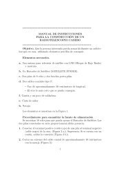
Figure 1 shows the total density distribution from the above components, and 

that excluding the molecular and cold HI. The latter is a first attempt to categorize 

the diffuse interstellar density, separating off material in dense regions occupying 

little of the volume. 

2.2. Vertical Gravity 

The vertical gravity at the Solar circle of Dehnen & Binney (1998) Galactic Model 2 

(DB2) was decomposed into its components, and the interstellar component, which 

in their model had a scale height of only 40 pc, was replaced by the integrated effect 

of the ISM distribution adopted above. The result was not strikingly dissimilar 

Figure 1 The distribution of interstellar hydrogen density above the Galactic Plane. The 

total is shown in blue, the warm diffuse component in red.


except close to the plane where the initial slope was reduced. A simple fit that 

agrees to better than 2% between z of 0 and 10 kpc is 

|g| =10 −9 cm s −2 {4.2[1 − exp(−|z|/165 pc)] + 4.1|z|/2 kpc} 

· (1 −|z|/27 kpc)/[1 + (z/6 kpc) 2 ] 1/2 . 



The first term on the first line represents the contributions of the ISM and 

disk stars, the second term is due to halo material, and the factors on the second 

line represent an accurate fit to the shaping apparently provided by the nonplanar 

geometry in the DB2 model. 

2.3. Interstellar Weight and the Vertical 

Distribution of Pressure 

Given the vertical density and gravity distributions, it is straightforward to calculate 

the weight of interstellar material above z, and thereby obtain an estimate of the 

vertical distribution of total pressure, p. Badhwar & Stephens (1977) made the 

initial bold steps in this direction, obtaining pressure values that were shocking at 

the time, but are now close to plausible after the revolution they precipitated. The 

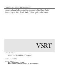
self-consistent pressure distribution for the conditions above is shown as the upper 

curve in Figure 2, assuming zero pressure at z = 10 kpc. The midplane value 

is 3.0 × 10 −12 dyn cm −2 ,orp/k B = 22,000 cm −3 K, where k B is Boltzmann’s 

Constant. 

2.4. The Thermal and Nonthermal Pressure Components 

Through the use of conventional values of the temperatures of the included interstellar 

components, their contributions to the spatially averaged thermal pressure 

can be estimated. The specific choices made here are 15 K for molecular gas, 80 K 

for cold HI, 5000 K for warm HIa, 8000 K for warm HIb, 7500 K for HII regions, 

and 9000 K for diffuse HII. As shown in Figure 2, the average thermal component 

is only 10% of the total in the midplane, and that percentage decreases outward. 

Note that this does not include thermal pressure of a high-temperature component 

that we have not yet discussed. 

In a study of this type, Boulares & Cox (1990) found that it was reasonable to 

suppose that there is rough equipartition between the nonthermal pressure forms; 

that assumption is now adopted as a hypothesis. As a result, the magnetic, cosmic 

ray, and dynamical pressures are each taken as one third of the nonthermal pressure 

of Figure 2, 0.92 × 10 −12 dyn cm −2 in the midplane. (Part of that dynamical 

pressure might be thermal pressure in the so-far ignored hot component.) For 

comparison, Ferrière quotes midplane values of 10 −12 and 1.28 × 10 −12 dyn cm −2 

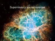
for magnetic field and cosmic rays, respectively. Assuming that the magnetic field 

is predominantly parallel to the plane allows calculation of the field strength versus 

z, as shown as the lower line in Figure 3. The midplane value is about 4.8 µG,

344 COX 



Figure 2 Comparison of the total (red) and volume average thermal (blue) pressure distributions, 

and their difference (black) interpreted as the nonthermal pressure. In this case, 

the total is taken from the weight distribution of the ISM. The thermal pressure neglects any 

contribution from the hot component. 

similar to current estimates of its strength (5 to 6 µG). The rms vertical velocity 

of the gas flows required to produce the dynamical pressure are moderate and of 

the order expected, rising from 6 km s −1 in the midplane. By the assumption of 

equipartition, they are close to the Alfven speed at all heights. 

The mean density sampled by cosmic rays is quoted as 0.24 cm −3 by Ferrière 

from measurements by Simpson & Garcia-Muñoz (1988) of the relative abundances 

of a radioactive isotope versus stable ones produced in the cosmic rays by 

spallation. By assuming that the local density of cosmic rays is proportional to the 

time they spend at a given height, and that they are equally likely to return to the 

Solar location from any height, the mean density sampled becomes just ∫ np CR 

dz/ ∫ p CR dz. For the above distributions of (total) density and nonthermal pressure 

the result is 0.19 cm −3 ,very similar to the measurement. If the particles diffuse 

outward, the mean density sampled by those that are found near the Sun would 

be somewhat higher. If the cosmic ray distribution is thicker, as found below, the 

value would be lower. 

The next comparison exposes a difficulty. The observed synchrotron emission of 

the Galaxy has been modeled, including its distribution above the plane in the solar




Figure 3 The vertical distribution of magnetic field strength. The red curve follows from 

assuming that one third of the nonthermal pressure of Figure 2 is magnetic, with the field 

parallel to the plane. The blue curve arises from the vertical distribution of the synchrotron 

emissivity, which implies that the rms field drops much more slowly with height. 

neighborhood. By assuming that the responsible cosmic ray electrons and magnetic 

field pressure track one another and the total nonthermal pressure p NT , Ferrière 

shows that the emissivity distribution behaves approximately as p NT (1/0.53) . Thus, 

the synchrotron distribution offers an independent test of the vertical structure of 

the nonthermal pressure. With Ferrière’s midplane values of magnetic and cosmic 

ray pressures and her quoted vertical distribution for the synchrotron emissivity, 

one obtains an estimate for the sum of these two pressures, which is compared to 

that found above in Figure 4. The figure also shows their difference. The difference 

in the midplane could easily be due to the uncertainties; but what is certainly true 

is that if the synchrotron emissivity distribution is correct, the magnetic fields and 

cosmic rays drop off much more gradually with height than found in our simple 

model. Returning to Figure 3, for example, the synchrotron-implied rms magnetic 

field is shown as the upper line.Itremains above 3 µG out to z = 2 kpc! If anyone

346 COX 



Figure 4 Comparison between the cosmic ray plus magnetic pressure estimated from the 

distribution of ISM weight (red) and that implied by the model adopted by Ferrière for the 

vertical distribution of the synchrotron emissivity (blue). The substantial difference is shown 

in black. 

is left who is inclined to believe that the galactic distributions of interstellar matter 

and pressure resemble that of a phonograph record, it is time to adjust that view 

to the extreme thickness of these distributions. 

The synchrotron emissivity implies that the cosmic rays and magnetic field 

persist to greater heights than would be inferred from the weight distribution of the 

interstellar matter considered so far. Facing this dilemma, Boulares & Cox (1990) 

showed that the high z nonthermal pressures could be coupled to lower z weight 

via magnetic tension, something like a suspension bridge. They proposed that the 

effective vertical magnetic pressure was (B 2 − 2B 2 z )/8π. With this explanation, 

the upper of the two curves in Figure 3 represents the rms B, whereas the lower 

represents the horizontal average of (B 2 − 2B 2 z )1/2 .Itwould require a substantial 

vertical component as one moves away from the plane. 

An alternative, proposed by both Badhwar & Stephens (1977) and Bloemen 

(1987), is to assume an additional very-thick-density component whose weight is 

sufficient to provide the additional pressure at high z. I will refer to this possibility 

as a coronal component. By assuming that the true pressure of cosmic rays and 

magnetic field is that advocated by Ferrière, I find that a component with density




(0.007 cm −3 )exp(–|z|/4 kpc) brings our pressure distributions into reasonable 

agreement. 

So far, I have neglected the potential thermal pressure of this coronal material. 

The calculations can be redone with any other assumption about this term. If it 

supplies the kinetic pressure component at z ∼ 1to3kpc (by hypothesis one third 

of the pressure not provided by the thermal pressures of the denser components), 

its temperature would be on order 3 × 10 5 K. If the temperature were about three 

times that, the material would be self supporting and not useful in solving the 

synchrotron emissivity distribution problem. In other words, it must not be too hot 

or it is not useful in this context. One must also take care that it does not excessively 

produce X rays. If the temperature actually were 3 × 10 5 K, OVI would be close 

to its peak concentration, about 0.25 of total oxygen. With an oxygen abundance 

of 5.6 × 10 −4 relative to hydrogen (Esteban et al. 2004, 2005), the total column 

density of OVI would be about 10 16 cm −2 , roughly two orders of magnitude more 

than is observed looking out of the galactic plane as we shall see below. If this 

coronal material were neutral, the column density of hydrogen would be about 

10 20 cm −2 , making it comparable to that in the denser components. If it were 

photoionized and at T ∼ 10 4 K, its emission measure looking out from the plane 

would be about 0.1 cm −6 pc, comfortably smaller than that of the Reynolds Layer 

(the thick HII mentioned previously), but its column density of electrons would 

be comparable (compare 0.007 times 4 kpc with 0.025 times 1 kpc). A modern 

plot of N e sin(b) versus z for high z pulsars (where N e is the column density of 

electrons) would be expected to test the existence of this coronal layer. I doubt it 

is there in this quantity. Interstellar material is surely present far from the plane of 

the Galaxy, but the quantity and properties of that material are heavily constrained 

by observations. 

3. SUPERNOVAE IN A HOMOGENEOUS MEDIUM 

This Section ignores nearly all inhomogeneity of the medium, asking how individual 

supernovae might evolve in it and what the observable consequences might 

be. It is a rough way to estimate the disruption they might cause, as well as the 

overall contributions to some observables that that fraction of the supernovae that 

avoid low-density regions might make. 

3.1. The Vertical Distribution of Supernova Rates 

The supernova rate distributions adopted by Ferrière (2001) for the Solar Neighborhood 

are, for Type I SNe (actually Ia), 

S I ≈ [7.3 kpc −3 Myr −1 ]exp(−|z|/325 pc) 

and for Type II (actually Ib, Ic, and II), 

S II = [50 kpc −3 Myr −1 ] ∗{0.79 ∗ exp[−(z/212 pc) 2 ] + 0.21 ∗ exp[−(z/636 pc) 2 ]}.

348 COX 



The latter was chosen to follow one of the models of pulsar birth sites of Narayan 

& Ostriker (1990). The term exp(–|z|/325 pc) in S I was chosen to represent the 

vertical distribution of stars. 

Ferrière further estimates that roughly 60% of the Type II SNe occur in groups, 

and that the range of group sizes is 4 to ∼7000 SNe with an average of 30. These 

groups are in the familiar association of OB stars, and lead to the growth of superbubbles, 

which evolve differently in volume occupation, pressure, and temperature 

from the remnants of the same number of supernovae occurring independently. As 

Iamnot comfortable with my understanding of that evolution, I will largely neglect 

superbubbles in the discussion below. That is not to say that they are unimportant, 

but that their actual effects on the observations I will discuss are difficult to estimate. 

So, the mindset is something like: This is what individual SNRs would likely 

do, at least approximately, and the presence of correlations in their occurrences 

will change things, downward by factors of less than two or upward by an unknown 

amount. 

3.2. A Simple Model of SNRs at High Temperature 

As long as neither radiative cooling nor external pressure has yet become important, 

a reasonable idea of the evolution and surface brightness of an SNR of explosion 

energy E 0 evolving in uniform density ρ 0 = mn 0 can be derived from the Sedov 

self-similar solution. The radius, expansion speed, post–shock temperatures, etc. 

are R = [2.025 E 0 t 2 /ρ 0 ] 1/5 ,v = dR/dt, T = (3/16) mv 2 /(χk B ), χ = (n + 

n e )/n, and m = ρ/n, while the luminosity is approximately 2.3 Vn 2 0 

L(T) where V 

is the volume. A reasonable fit to the nonequilibrium cooling coefficient is L(T) ≈ 

α T −1/2 , where α ≈ 10 −19 erg cm 3 s −1 K 1/2 (the Kahn approximation; for more 

detailed accounts see Cox & Anderson 1982 for its usefulness and Smith et al. 1996 

for its accuracy). The “2.3” in the luminosity derives from the average compression 

of the material. (Note: n = n H + n He = 1.1 n H ,except in Sections 2 & 4 where 

n = n H .) 

Two further pieces of information are useful when considering X-ray emission, 

first that the average surface brightness is the luminosity divided by πR 2 . This is 

often estimated in terms of the average “emission measure” ∫ n 2 e dl, which for this 

simple remnant model is EM ∼ 2.3 (4/3) n 2 0 

R. The second item is that Snowden et 

al. (1997) provide the count rate per emission measure in various ROSAT bands. 

From their figure 9, for example, a RS plasma model at 10 6 K with no intervening 

absorbing material and an emission measure of 1 cm −6 pc is expected to provide 

roughly 1.5 × 10 5 [10 −6 counts s −1 arcmin −2 ]intheR12 ( = R1 + R2) energy 

band. This response function depends on the atomic physics and abundances used. 

Once again, I will simply adopt the curves of Snowden et al. (1997) as a fiducial 

set, with concerns about details beyond the present scope. 

Because I am first concentrating on the potential X-ray emission by remnants, 

it is useful to describe their properties as a function of the post–shock temperature, 

T 6 ,inunits of 10 6 K. Using E 51 as the explosion energy in units of 10 51 ergs, from 

above one can derive the following:


R ≈ 19.3 pc[E 51 /(n 0 T 6 )] 1/3 , 

t ≈ 28,000 years (E 51 /n 0 ) 1/3 /T 5/6 

6 

, 

E rad /E ≈ 0.064 (E 51 n 2 0 )1/3 /T 7/3 

6 

(fraction of energy radiated above T 6 ), and 

EM ≈ 59 cm −6 pc n 5/3 ( ) 1/3. 

0 E51 /T 6 



If the rate of supernova occurrences per unit volume, S, is expressed in units of 

SN (kpc) −3 (Myr) −1 , the fractional volume occupation of remnants hotter than T 6 

is given by 

f ≈ 3.83 × 10 −7 S(E 51 /n 0 ) 4/3 /T 11/6 

6 

. 

In what follows, I shall assume that all supernovae occur with 10 51 ergs, and 

lose little of this (to cosmic ray acceleration, for example) prior to entering the 

adiabatic phase. (This is probably an upper limit.) The total SN power density at 

midplane is then 6.15 × 10 −26 erg cm −3 s −1 , and the total power per unit area 

(for both sides of the disk) is 1.05 × 10 −4 erg cm −2 s −1 . 

3.3. The Average Interstellar X-Ray Emissivity 

from Supernova Remnants 

Using these distributions and the result above for the fraction of energy radiated 

at temperatures T 6 and above, one can calculate the local volume average emissivity 

of the population of supernova remnants, assuming that at each height, z, 

all of the remnants (ignoring clustering) evolve in the average density. Given the 

extreme inhomogeneity of the ISM, this is a peculiar thing to do, but it provides 

a sense of the orders of magnitudes anticipated for various quantities and their 

variation with z. For T 6 = 1, this was done for two cases, supernovae evolving 

in the total average density, and instead evolving only in the average of the 

intercloud or “diffuse” component. At higher temperatures, the results must be 

scaled by T −7/3 

6 

.For the two cases, the midplane emissivities are 4.4 × 10 −27 

and 1.4 × 10 −27 erg cm −3 s −1 , while the total vertically integrated efficiency 

for radiation of SN power above 10 6 Kis3.2% for interaction with the full average 

density and 1.6% for interaction with the diffuse gas only. We recover the 

usual result that SNRs in uniform density radiate very little of their energies in 

X rays; most of their emission comes later at lower temperatures, in the EUV 

(hard ultraviolet). 

The radii of the remnants at 10 6 K are moderate in the midplane (18 to 33 pc) 

but increase to 48 pc at z = 400 pc and 78 pc by z = 1 kpc. The fraction of 

the volume occupied by remnants with T 6 > 1isvery small; even if they interact 

only with the diffuse gas it is only about 2 × 10 −4 for |z| < 1 kpc. The chance of 

encountering a hot remnant on any given line of sight is extremely small.

350 COX 



Suppose, however, that one overall effect of interstellar inhomogeneity is to 

further homogenize the X-ray emission of the Galaxy, without substantially altering 

its average rate. One then expects the ROSAT R12 band, sensitive to gas at 

roughly 10 6 K, to be responding to a surface brightness, from data given above, 

of about 2% of half of 1.05 × 10 −4 erg cm −2 s −1 , looking out of the plane of 

the Galaxy. Using the previously mentioned Kahn approximation to the cooling 

coefficient, the corresponding emission measure is 3.4 × 10 −3 cm −6 pc. The remarkable 

coincidence is that this is roughly the value ascribed to the Local Bubble 

to produce the diffuse 1/4keV X-ray background. 

We can similarly estimate the M band or R45 count rate, sensitive to ∼3/4 

keV Xrays. By converting the E/E formula to a probability distribution function 

in 〈n 2 e 〉 with T, and invoking the ROSAT sensitivity to gas between 2.5 × 

10 6 and 6.3 × 10 6 K, my estimate of the midplane R45 count rate achieved in 

1 kpc (approximately one optical depth) is 200n 2/3 

0 

[10 −6 counts s −1 arcmin −2 ]. 

For the total and diffuse midplane densities, this ranges from 220 down to 66 in 

these units. Again we have an amazing coincidence that these estimates bracket the 

observed diffuse count rate of roughly 120 in R45 in the midplane. It appears that 

the diffuse component X rays we observe are comparable to those expected from 

the Galactic population of individual SNRs, but somehow homogenized. Without 

that homogenization, the emission would be confined to small bright remnants. 

Some of it, of course, is. 

3.4. Porosity and OVI 

The notion of supernova-generated porosity of the ISM was introduced by Cox 

& Smith (1974). The basic idea is that if one calculates how remnants would 

evolve independently of one another, and from that the total volume fraction of 

the ISM the population of remnants would occupy, then one has a measure of 

the likelihood that remnants will or will not evolve independently. That volumefraction-assuming-independence 

is called the porosity, q. If q is much less than 

1, it is safe to assume that remnant interactions are rare and that the remnants do 

indeed occupy a volume fraction q of the medium. If q is not small, it is less clear 

what happens. Remnant interactions are important. Some supernovae would occur 

in very-low-density regions already evacuated by previous remnants, or would 

occur in a denser region but break into a low density one during their evolution. 

The medium evolves toward some new configuration in which low-density and 

high-temperature regions are common. The critical porosity for this change in 

configuration of the medium has not yet been established and probably will depend 

sensitively on the details one assumes about the medium and remnant evolution 

at the outset. Smith (1977) presented an attempt to find this critical porosity, with 

the result that, if it existed, it was larger than supposed by Cox & Smith (1974). 

The result is derived from a specific and complex view of how remnants interact 

with one another and their environment. 

McKee & Ostriker (1977) presented an estimate of q for the ISM and found 

that it was very large, demanding restructuring be present. Slavin & Cox (1993)




concluded that the McKee & Ostriker estimate was too large, for several reasons, 

and that the porosity of the medium outside superbubbles could well be small. 

Subsequent efforts have been made to calculate the porosity due to superbubbles 

separately from that of the medium outside (see Ferrière 2001). We now evaluate 

the porosity anticipated in our homogeneous medium model. 

If the volume of the low-density cavity of a remnant is V(t), and the rate of SNe 

per unit volume is S, then the porosity defined above is 

∫ 

q = S V(t) dt, 

where the integral is over the entire lifetime of the remnant cavity. Various attempts 

to estimate the V(t) function from analytical considerations have not been very 

successful, but one set of hydrodynamic calculations was made by Slavin & Cox 

(1992, 1993) to learn how remnants might evolve at late stages. Their work made 

specific approximations to the role of magnetic pressure in the ISM and thermal 

conduction within the hot gas, approximations that might not satisfy all tastes, but 

which are clearly described and reasonably motivated. They fit their results for 

varying density, explosion energy, and external pressure with the expression 

q = 0.176 S −13 E 1.17 

51 n−0.61 0 

(10 −4 p/k B ) −1.06 , 

where S −13 is the SN rate in units of 10 −13 pc −3 yr −1 . (Ferrière’s total midplane rate, 

including clustered SNe, of 57.3 corresponds to S −13 = 0.573.) In this equation, 

pisthe external pressure within which the remnants are evolving. It is reasonable 

to assume this is roughly half the total pressure, taking old remnants to be largely 

transparent to cosmic rays and neglecting some of the dynamical pressure of the 

medium as well. Using our results for the distributions of SNe, density, and pressure 

(specifically that of Figure 2), again with E 51 = 1, we arrive at the porosity versus 

height curves shown in Figure 5, the lower curve for all SNRs evolving in the full 

density, the upper for all SNRs evolving in the diffuse mean density. 

The two porosity curves differ by a factor of 3 in the midplane, but converge at 

higher z where the cloud component is largely absent. The values are substantial, 

∼0.25 from z = 250 to 700 pc, particularly in light of the Cox & Smith (1974) 

suggestion that above a rather modest porosity there might be a tendency for 

the SNe to occur within existing low-density cavities and promote the growth 

of a pervasive phase of hot gas, their tunnel network (but see also Smith 1977). 

(The reason that high porosity is consistent with the very-low-filling factors for 

hot remnants in Section 3.3 is that most of ∫ Vdtcomes from the late stages of 

evolution, during further expansion after cooling has occurred, and when the SNR 

bubble is collapsing.) 

Porosity, though useful as a theoretical tool, is not an observable phenomenon. 

On the other hand, the mean density of an ion, O +5 , present during the late evolution 

of remnants, is observed, and can be used as a direct test of whether this 

porosity calculation has any validity. We shall see that, in fact, the OVI density 

and distribution calculated next are very much in line with the observations.

352 COX 



Figure 5 The distribution of SNR-induced porosity, assuming that all SNe occur in the 

total average density (blue)ordiffuse density (red). 

In the same set of calculations, Slavin & Cox (1993) also fit their results for the 

OVI dosage of their remnant evolutions, where dosage is defined as D = ∫ N(OVI) 

dt and N(OVI) is the number of O +5 ions in the remnant as a function of time. 

Their fit was 

D OVI = 8.13 × 10 60 E 1.11 

51 n−0.76 0 

(10 −4 p/k B ) −0.16 ion years. 

The corresponding mean density of OVI ions is 3.4 × 10 −69 S −13 D OVI . Shelton 

(1999) considered three remnant evolutions at densities substantially lower than 

those sampled by Slavin & Cox. Using the parameters of Shelton’s remnants, it is 

found that the Slavin & Cox formula underestimated her OVI dosages by factors 

ranging from 1.34 to 1.5. The agreement is thus well within the range of uncertainty 

of the many parameters employed in making these estimates. 

Once again using our vertical structure, this mean OVI density calculated versus 

z from the above formula is shown in Figure 6. The midplane range for the two 

assumed densities is 1.4 × 10 −8 to 5.4 × 10 −8 ion cm −3 . The column densities 

perpendicular to the plane are 0.82 × 10 14 to 1.0 × 10 14 cm −2 , per side.




Figure 6 The distribution of average interstellar density of OVI, assuming that all SNe 

occur in the total average density (blue) ordiffuse density (red). The observed midplane 

value is about 1.7 × 10 −8 cm −3 . 

The observed average midplane density of OVI is approximately 1.7 × 10 −8 

cm −3 (Bowen et al. 2005), very similar to the above value from all SNe interacting 

with the total density. A similar number would be found by taking only 

the SNe outside groups and using the diffuse ISM density. Attempts to measure 

the column density perpendicular to the plane have been made by Savage et al. 

(2003), who find the OVI to be very patchy with values ranging from 0.6 × 

10 14 to 3 × 10 14 cm −2 ; the larger values are prevalent in the north. The southern 

and northern median values are 1.1 × 10 14 and 1.8 × 10 14 cm −2 . The values 

of our model above lie at the low end of the observed range, and do very well 

at reproducing the median in the south. Patchiness and edge brightening of the 

OVI-bearing volumes can lead to individual sight lines with column densities 

well above the mean. On the whole, the model predictions are very close, certainly 

within the uncertainties of the calculation. Reference to the lower curve 

of Figure 6 suggests that estimating a scale height for this material could be 

misleading. The modeled mean density rises considerably away from the plane 

before it drops again. One might describe the thickness of the layer as about 1 kpc 

rather than the 2 kpc obtained by dividing the vertical column by the midplane 

density.

354 COX 

As will become apparent later, the problem with OVI is not how to get as much 

as is seen, the problem is always how to keep from getting too much. The simple 

model presented above shows that just about the right amount would derive from 

Slavin Bubbles, the old cooling cavities of SNRs evolving in the warm intercloud 

environment. As we examine the ISM and discover its large volumes of much lower 

density, it becomes unclear how to avoid having much larger quantities of OVI. 



4. THE TWO-PHASE MEDIUM REVISITED 

4.1. Basics 

The fundamental purpose of the modern two-phase calculations is to explore the 

segregation of the bulk of the interstellar material into cold and warm components. 

Its methods are to assume a density, calculate the ionization and electron density at 

that density, along with the charge state of the PAHs (poly aromatic hydrocarbon 

molecules), and find the self-consistent thermal balance between the photoelectric 

(and other sources of) heating and radiative cooling. The result is an equilibrium 

T(n). From that, one calculates the thermal pressure function p Th (n). The details 

are sensitive to a variety of input parameters. The typical result is a sinuous curve 

for which there is a range of p Th over which the density is triple-valued at constant 

pressure. With that curve in hand, one examines it for the possibility of having 

clouds and intercloud gas at the same thermal pressure with a thermally unstable 

regime between them, the phase segregation. 

There is not a universal p Th (n) curve; the heating rate varies with galactic 

location and time (e.g., Parravano, Hollenbach & McKee 2003), and with the 

opacity between the gas parcel of interest and the sources of radiation providing 

the ionization and heating. In what follows, a representative example for the Solar 

Neighborhood is taken from Wolfire et al. (2003). It is shown, somewhat decorated 

with auxiliary information, in Figure 7. 

The lower curve, shown in three colored segments, is the original; the upper 

(dotted aqua) curve shows the approximate effect of having a heating rate about 

10 times higher. Also shown are the approximate weight per unit area of the 

interstellar medium (dashed black), the probable typical magnetic pressure close 

to the galactic plane (dashed orange), and a region bordered by a rectangle to be 

discussed later. 

The p Th (n) curve has several familiar features, described in the classic paper 

on this subject by Field, Goldsmith & Habing (1969). These include separate 

branches for warm intercloud (red) and cold cloud (green) components, a maximum 

intercloud thermal pressure (4400 cm −3 K for the curve shown), a minimum 

cloud thermal pressure (1700 cm −3 K for this example), and a range of density 

(0.8 to 7 cm −3 ), or more fundamentally temperature (roughly 270 to 5500 K), 

between these two (blue) that is regarded as forbidden in equilibrium because 

at constant thermal pressure it is thermally unstable. In the unstable region, gas 

slightly above the curve is too hot for its density and cools. But at constant thermal




Figure 7 The Two-Phase Medium thermal pressure versus density curve is shown in the 

red-blue-green curve. The red segment is the thermally stable warm component, the green the 

corresponding stable cold component, and the blue the thermally unstable regime. The black 

dashed line is the total midplane pressure, the orange dashed line represents the magnetic 

pressure, the dashed aqua line shows how the p(n) curve shifts when the heating rate is raised 

considerably, and the dashed purple rectangle outlines the regime of essentially zero bulk 

modulus. 

pressure, cooling moves it to the right, to higher density, taking it further from 

the curve and making it cool faster, until it reaches the stable cloud branch. 

Similarly, gas slightly below the curve has excess heating and at constant thermal 

pressure moves horizontally to the left until it joins the stable intercloud 

component. 

4.2. Less Familiar Aspects of the p Th (n) Diagram 

For the standard curve, the mean midplane interstellar density in the Solar Neighborhood 

(slightly over 1 cm −3 )isinthe unstable regime. This appears to guarantee 

that both the cloud and intercloud branches will be populated. 

A significant portion of the cold-cloud branch lies below the total midplane 

pressure (the weight per unit area of the ISM), and even below the mean magnetic

356 COX 



pressure that is about a third of the total. This appears to allow the cold-cloud 

population a comfortable existence. The total pressure is more than enough to 

hold them together, and whatever thermal pressure they lack can be augmented by 

sufficient internal magnetic pressure. 

Note however that with the higher heating rate sketched, both of the above 

conditions would change. The current mean density would then be well into the 

intercloud branch, while even the minimum allowed thermal pressure of a cold 

cloud would be close to the total available pressure and well above the thermal 

pressure that any abutting intercloud gas (at the mean density or lower) might have. 

This combination assures that clouds would be very difficult to form or sustain, 

while the medium could rest quite comfortably in a fully warm component. 

With no cold HI component, it might be very difficult to make molecular clouds; 

if so, the star formation rate would decline with time. As the photoelectric heating 

relies predominantly on radiation from the younger stars, heating would also 

decline until clouds were once again stable. (This is a situation that Antonio Parravano 

has been exploring since at least 1987.) Thus, the ability of dense clouds 

to exist at thermal pressures available in the medium appears to set an upper limit 

on the mean star formation rate. This is a complicated subject dependent on grain 

and PAH properties, on the local ionizing radiation field, on the scale height of the 

warm component (as it basically provides the weight determining the midplane 

pressure), and even on the absolute and relative gas-phase abundances of carbon 

and oxygen. But properly understanding it might lead to a prescription for a selfconsistent 

star formation rate, given the total pressure (which likely also depends 

on that star formation rate). 

One of the most interesting features of p Th (n) is that over a density range of a 

factor of 350, from 0.2 to 70 cm −3 , the thermal pressure variation is less than a factor 

of three. In Figure 7, this region is shown enclosed by a dashed purple rectangle. 

It is a regime in which the thermal pressure offers essentially zero bulk modulus. 

This means that if, for some reason, the ISM had a totally random distribution 

of densities within this range, the corresponding distribution of thermal pressures 

would be observationally indistinguishable from one in which thermal pressure 

had an active role in arranging things, except there would be no range of forbidden 

densities. Most of the remaining points have to do with how this might be related 

to the actual interstellar situation. 

A reasonable first order approximation to interstellar conditions (near the plane) 

is to think of the sum of thermal and magnetic pressure being constant at roughly 

half the total pressure. This assumes that the cosmic ray component is uniform and 

that the dynamical component is roughly so as well. For the Solar Neighborhood, 

that sum should be on the order 1.5 × 10 −12 dyn cm −2 or 11,000 cm −3 K. (This 

is not a firm number; I have elsewhere quoted it as 20,000 cm −3 Konlyafew 

years ago. The observations underlying it have uncertainties, and the role of the 

dynamic pressure component is situation-dependent.) This number then provides 

an upper limit on the thermal pressure. In regions that are quiescent, in pressure 

equilibrium with their surroundings, but in which abundant thermal energy




has caused enough expansion that the magnetic field pressure is substantially reduced 

from normal, this pressure would be almost entirely thermal. The expected 

range of thermal pressures in the quiescent cloud component of the ISM should 

then lie between the minimum cloud pressure, 1700 cm −3 K, and the upper limit, 

11,000 cm −3 K. This is comfortingly similar to the range of most observations reported 

by Jenkins & Tripp (2001). At the low-density end of the diagram, however, 

the allowed range of thermal pressures is much broader, from zero to the upper 

limit. 

The previous two paragraphs have suggested that the small variation in thermal 

pressure between regions of differing density can be compensated by slight 

changes in the somewhat stronger magnetic field pressure. This is true when establishing 

pressure uniformity across the magnetic field lines, but equilibrium 

parallel to the field cannot be established in this way. So, one might still imagine 

that thermal pressure has a role in arranging things parallel to the field and will 

lead to cloud–intercloud segregation and the disappearance of material from the 

thermally unstable regime. The fundamental flaw in this idea is not recognizing 

the importance of the extreme density difference between the cloud and intercloud 

components. The differential is two to three orders of magnitude. If thermal pressure 

is to move material from intercloud to cloud component, parallel to the field, 

then to build a cloud of 1 pc extent, it must collect intercloud material from several 

hundred parsecs. Even at a relative velocity of 10 pc/Myr, the approximate sound 

speed in the warm component, this requires several tens of Myr, a long time to 

imagine interstellar quiescence is appropriate. The converse process, in which a 

cloud expands into a low-pressure region to fill it with intercloud material, takes 

even longer at the lower sound speed of the cloud. It appears to me, and several 

others who have begun modeling gas in transition (e.g., Vazquez-Semadeni et al. 

2003), that dynamics is all-important in deciding what densities will be where; 

thermal instability has a decidedly secondary role. At the high densities of cold 

clouds, the temperature and ionization adjust rapidly to the equilibrium, producing 

results consistent with the p Th (n) equilibrium, but at lower densities the temperature 

and ionization can take a long time to adjust, and between the high- and lowdensity 

components, adjustment to uniform thermal pressure takes much longer 

yet. 

4.3. Surprises of Two-Phase Modeling 

A number of dramatic consequences follow from the above discussion. They include 

the following: 

(1) Thermal pressure in diffuse HI in the Galaxy has little dynamical effect. 

In quiescent regions, it is usually several times smaller than the magnetic 

pressure, so thermally driven flows, to the extent they exist, will tend to be 

along the field, one dimensional. In addition, these 1D transitions between 

components take longer than the timescale for the external alterations of 

their environment.

358 COX 



(2) Zero thermal pressure is allowed at low densities. Such regions occupied by 

their full complement of cosmic rays and magnetic field require no additional 

thermal pressure. 

(3) Over a very wide range of HI densities, the limited range of the equilibrium 

thermal pressures makes thermal pressure look important even when it is 

not. 

(4) In quiescent regions, the value of the magnetic field should vary little with 

density—a little low where thermal pressure is high, a little high where 

thermal pressure is low. 

(5) The forbidden range of n,T is probably common, present in the slow transition 

between stable components, or just put there by dynamical events. 

(6) If cold clouds must exist for star formation to occur, then photoelectric 

heating provides a feedback loop for setting an upper limit to it for a given 

pressure. 

4.4. Filling Factors of the Denser Components 

From the thermal pressure curve, along with the mean thermal pressures found in 

clouds, it has become customary to assume that the equilibrium thermal pressure 

of HI is about 3000 cm −3 K. I adopt 2800 cm −3 K. From Figure 7, the cloud and 

intercloud components then have densities and temperatures of 30 cm −3 ,93K, 

and 0.36 cm −3 , 7800 K, respectively. I will make these choices, with one exception. 

I regard the density of 1 cm −3 to be more likely for a significant fraction 

of the component I have referred to as warm HIa, because in experiments with 

the transition between clouds and intercloud components, it seems to be true that 

material often spends a great deal of time in the vicinity of the density at which 

the intercloud pressure is maximum. I will therefore assume 30 cm −3 for the local 

density of clouds, 0.36 cm −3 and 1 cm −3 each for half of component HIa, and 

0.36 cm −3 for all of component HIb. I will neglect the filling factors of the molecular 

and classical HII regions, which are very dense or contain little material, 

respectively. I will further assume that the diffuse HII gas is the ionized part of 

HIb and that the material has expanded slightly laterally, with B ∝ n, as the temperature 

increases to 9000 K and the number of thermal particles doubles in the 

ionization. Constant thermal plus magnetic pressure then results in a density of 

0.3 cm −3 for the diffuse HII. That is, the thermal pressure in the ionized gas is 

somewhat higher, and the magnetic field somewhat lower, than in the warm HI 

with this assumption. It is a rough estimate, but embodies the basic idea. 

From the mean densities in the midplane given earlier, the filling factors (with 

considerable uncertainty) are then 0.013 for cold HI, 0.194 for warm HIa, 0.174 

for warm HIb, and 0.083 for diffuse HII. The grand total is roughly 46%. The 

implication is that something like half the volume of interstellar space might have 

much lower densities than that in the components above. As it is almost certainly 

ionized, that component’s mean density must be less than something like


0.02 cm −3 in order not to contribute substantially to the electron density measured 

via pulsar dispersions. The only clear alternative is that the warm components fill 

nearly all of the space, with a lower density than estimated above, about 0.2 cm −3 , 

and this is inconsistent with the inhomogeneity described in the following section. 

5. LARGE-SCALE INHOMOGENEITY 



Segregation of the matter into cold and warm components is not the only source of 

inhomogeneity in the ISM. In this section we consider the arm/interarm contrast, 

the observations indicating that there are large cavities and tunnels of very low 

density in the ISM and the observed distribution of the denser matter. 

5.1. Spiral Arm Contrast 

The interstellar medium is expected to have a certain amount of large-scale inhomogeneity 

just from dynamical events. Consider first the anticipated contrast between 

arm and interarm regions. In a recent single-phase MHD model of Galactic ISM 

dynamics, for example, Gomez & Cox (2004) found column-density contrasts of 

about a factor of three. My impression is that in the Milky Way the denser components 

probably do have contrasts between three and five, but that the contrast is 

likely much less for the more diffuse components. 

I bring this up because our fiducial calculation of the weight of the ISM used 

estimates of the mean densities of the various components, with different sampled 

regions contributing to the estimates for different components. In addition, if all 

components had contrasts of three, one might suppose that there would be similar 

differences in the arm and interarm pressures. One of the tests made by Gomez & 

Cox dealt with this question, comparing the ISM weight and midplane pressure 

around the Solar circle in their model (see their figure 12). The averages of the two 

were equal, but the weight per unit area was about a factor of four higher in the 

arms than interarm regions (higher column density and thicker distributions). But, 

the midplane pressure variation was closer to a factor of two, with twice the spatial 

frequency, having peaks in both arms and interarm regions. The principal cause 

for this difference was vertical dynamics, i.e., the bouncing of high z material. The 

bottom line to this diversion is that the pressure we previously calculated likely has 

significant variations about it associated with the arm/interarm contrast, perhaps 

with about a factor of two in range. Students of radio continuum emission could 

probably offer a better estimate. 

5.2. Cavities 

Another large-scale dynamical activity is the formation of superbubbles by the 

winds and supernovae of OB associations. Several of these are known nearby, 

including the Orion-Eridanus and Loop I superbubbles. It has been estimated 

that the diffuse interiors of the collection of these bubbles occupy something like

360 COX 



20% of the volume in the midplane (Heiles 1990, Ferrière 1998). In each case, 

the remainder of the OB stars responsible for the bubbles is plainly seen. But, 

there is another considerable cavity for which there is no clear association of 

young stars, the Local Cavity surrounding the Solar location, to which we now 

turn. 

The most recent report of a very ambitious effort to map the density distribution 

in the Solar vicinity is provided by Lallement et al. (2003). Column densities 

in NaI are reported for about 1000 stars, and from them, maps of the spatial 

distributions of column density and density of cold gas within the nearest few 

hundred parsecs of the Sun are derived. There is a very-low-density region around 

the Sun, with the nearest high-density gas about 55 to 60 pc away in the first 

quadrant. In other directions, the dense “wall” of the Local Cavity is much farther 

away. The cavity is essentially open at high positive and negative latitudes, with 

tunnel like extensions in the disk in a variety of directions, some seeming to connect 

our cavity with others nearby. The authors’ view is that other nearby cavities are 

younger higher pressure regions that are forcing the walls toward us, squeezing 

our older lower pressure cavity. Perhaps their future studies of the motions of 

the intervening material will confirm this squeezing. In any case, there is a very 

large irregular hole in the distribution of gas near the Sun, a hole that appears to 

have narrower connections to more distant voids and that extends well out of the 

plane. 

Lallement et al. show an inner contour that they say corresponds to a column 

density of 2 × 10 19 cm −2 of hydrogen. In a distance of 60 pc, the mean sightline 

density is 0.1 cm −3 . But the mean densities to individual closer stars are often 

much lower, such that the column density of the contour is acquired only as the 

wall is approached. On the other hand, their method is sensitive only to cold dense 

gas, and could miss the warmer low-density material. Such material is, in fact, 

found in the spectra of stars close to the Sun, the Local Fluff, but it appears to have 

alow filling factor in the cavity as a whole. 

Much of the 1/4 keV soft X-ray background appears to derive from within 

roughly one million Kelvin gas occupying at least part of the Local Cavity. This 

hot region is generally referred to as the Local Bubble, or Local Hot Bubble. What 

I think I know about this can be found in Cox & Reynolds (1987), Cox (1998, 

part of a whole conference volume on the subject; 2004), Cox & Helenius (2003), 

and Florinski et al. (2004). I will just mention some recent developments. Further 

discussion and references appear also in Lallement et al. (2003). 

In brief, the 1/4keV soft X-ray background is now known to have three source 

components: heliospheric emission from charge exchange of highly ionized Solar 

wind particles with interstellar neutrals penetrating into the Solar System, thermal 

emission from the Local Hot Bubble, and additional thermal emission from more 

distant hot gas regions within the thick interstellar disk. The origin of the Local 

Cavity has been speculated upon, but is unclear. The true story of the Local Bubble 

emission will remain uncertain until we have spectral resolution that tells us 

precisely what stages of ionization of what elements are responsible for the X-ray


emission and we can separate the heliospheric contribution spectrally. The Local 

Fluff has interesting stories to tell, but is not yet fully understood. Among other 

things, it has a pressure problem. The measured thermal pressure in the Local 

Fluff is only about one fifth of that inferred for the hot gas surrounding it. If the 

difference is made up by magnetic field, models imply that, contrary to fact, the 

termination shock of the Solar wind should already have been encountered by 

Voyager I, unless the field is locally parallel to the relative motion of the Sun and 

Local Cloud (Florinski et al. 2004). 



5.3. Two Other Examples of Non-OB Association 

Cavities, and Two More Tunnels 

There are two other rather large regions observed to be emitting 1/4keV X rays but 

which, like the Local Bubble, are not superbubbles. One of these is the MonoGem 

Ring, the other the higher latitude Draco enhancement. The MonoGem Ring is a 

round feature 25 ◦ in diameter, centered at l = 203 ◦ ,b =+12 ◦ . Its brightness 

in the ROSAT R12 band is about 420 (10 −6 counts s −1 armin −2 ) after correction 

for moderate intervening absorption. Using the previously mentioned 1.5 × 10 5 

conversion from EM to R12 units at 10 6 K, one arrives at the implied emission 

measure of 2.8 × 10 −3 cm −6 pc. Using our Sedov SNR model, one arrives at the 

anticipated EM of 59 n 0 5/3 for E 51 = T 6 = 1. The required value of n 0 is then 2.55 

× 10 −3 cm −3 .With that same model, the radius and age are 141 pc and 2 × 10 5 

yrs. With a post–shock temperature of 10 6 K, assumed above and implied by the 

X-ray emission, the post–shock pressure would be 4n 0 χk B T s ∼ 3 × 10 −12 dyn 

cm −2 , high enough that further expansion would be expected if the cavity is large 

enough. The angular diameter implies a distance of about 640 pc. The object has 

been modeled more carefully by Plucinsky et al. (1996) with similar conclusions for 

E 51 = 1. Lower energies would place the object closer, making it smaller, younger, 

and evolving in slightly higher density (see their table 7). Stating that another 

way, if this object is a few hundred parsecs distant, it is a couple of hundred 

parsecs across, contains of order one supernova worth of thermal energy, and has 

an average density between about 3 × 10 −3 and 5 × 10 −3 cm −3 .Itistherefore in 

an exceedingly large cavity with a very low density, a cavity not associated with a 

superbubble. 

The Draco enhancement in the 1/4 keV background is a bright region with a 

diameter of roughly 15 ◦ centered at about l = 95 ◦ ,b =+38 ◦ .Itisshadowed 

by much of the HI along the line of sight, but its surface-brightness contribution 

has been separated from the Local Bubble emission by Snowden et al. (1998), 

and corrected for the absorption. Its R12 brightness before absorption is about 

2600 (10 −6 counts s −1 armin −2 ), implying an emission measure of 0.017 cm −6 

pc. Following the above procedure with the simple Sedov model, again assuming 

E 51 = T 6 = 1, we are led to n 0 = 7.5 × 10 −3 cm −3 ,R = 98.5 pc, age = 1.43 × 

10 5 years, distance = 750 pc, z = 460 pc. In this case, the post–shock pressure is 

about 9 × 10 −12 dyn cm −2 so that the shock is still strong. It is a quite reasonable

362 COX 



candidate for being a supernova remnant fairly high up in the thick galactic disk. 

Shelton (1999) has provided detailed models for such objects. 

One might wonder about the likelihood of supernova remnants as young as 

this at high latitude. But, integrating Ferrière’s SN distribution in a cone about the 

zenith with opening angle θ,wecome to the total SN rate on one side of the plane 

of 5.8 tan 2 (θ) Myr −1 , most of them between 500 and 1500 pc off the plane. As 

the Draco enhancement is at θ ∼ 52 ◦ ,weexpect 1.4 remnants at this latitude or 

higher with ages of 1.43 × 10 5 years or lower. So, what we see, one, is plausible. 

The more surprising part is that the size is again large and the mean density once 

again quite low. From Figure 1, we find that the mean density 500 pc off the plane 

should be about 0.04 cm −3 and that it does not drop to 7.5 × 10 −3 cm −3 until z 

∼ 1500 pc. 

An important point is that the density in these two regions, like that in the Local 

Cavity, was low prior to the assumed supernova explosion that brought them up 

to 10 6 K. The temperature must also have been low, or we would not need the 

supernovae to heat them. 

One last thing. Plucinsky et al. (1996) discuss the observed column densities 

toward stars in the direction of the MonoGem Ring. In their table 4, several stars 

with quoted distances of 700 to 2300 pc have total column densities in the range 

1.1 × 10 20 to 2.3 × 10 20 cm −2 .Acolumn of 10 20 cm −2 in 1000 pc has a mean 

density of only about 0.03 cm −3 .Itisanexample of those directions for which, over 

vast distances, very-low-density lines of sight are found, as discussed by Lallement 

et al. (2003). Another was recently rediscovered by Madsen & Reynolds (2005) 

toward the inner Galaxy,a6kpc line of sight toward Scutum with a mean density 

of about 0.16 cm −3 . This mean is not so extraordinarily low, but is likely made up 

of stretches with much lower density between those with more normal values (and 

which show up as velocity peaks in the HI profile). This case is exceptional in its 

great length. 

In summary, there are very large regions of interstellar space with very low 

density, many of which are not in currently active superbubbles, and some of 

which are apparently not hot (so that they can be reheated by supernovae to appear 

as bright regions in the soft X-ray sky). Others could be too hot and diffuse to 

make their presence known via X-ray emission. 

5.4. How is the Matter Arranged? 

We have so far considered only the photographic negative view of the structure of 

the ISM, where material is not. There are a few things to say about how material 

is arranged where it is found, the photographic positive of the picture. My opinion 

is that the best idea of this is found by actually looking at pictures. Examine 

the 21-cm survey pictures, IRAS pictures, Hα pictures, and optical continuum 

pictures. What do you see? The distribution appears to be dominated by many 

large-scale structures. There are loops, filaments, and shells galore, as well as some 

concentration into the arm structures, though it is sometimes difficult to discern.




There is also some information about the relative locations and geometries of 

the various components. Heiles & Troland (2003) reviewed the HI information. I 

think a fair summary is that warm low-density HI is arranged in large sheets, with 

some considerable thickness. Within these sheets, there is filamentary structure, 

and denser cold subsheets and filaments, the cold cloud material of low volume 

filling factor. With increasing distance from the plane, the relative proportions 

shift, with the cold component less prevalent. This is mirrored in the differences in 

the scale heights of the two introduced at the beginning. At very high |z|, the cold 

component tends to peter out, but in the inner Galaxy, at least, Lockman (2002) finds 

there are small fragmentary bits of warm HI, some of which have cold cores. What 

about the molecular clouds and their complexes? I do not pretend to know anything 

about these, but my impression is that, except near the Galactic Center, they are 

found only in regions where there is a large amount of HI in the neighborhood. 

Various excuses are given for this—shielding from the UV, gravitational binding, 

compression in the spiral arms, etc. An outsider gets the impression that they are 

just another natural form of condensation that occurs when a lot of material gets 

close together. There is heated discussion about how long they exist and how long 

it takes them to form stars. 

6. LIMITS ON 3 × 10 5 AND 3 × 10 7 K GAS IN THE ISM 

6.1. The OVI Constraint on 3 × 10 5 K Gas 

The average midplane density of O +5 is about 1.7 × 10 −8 cm −3 (Bowen et al. 

2005). The abundance of oxygen relative to hydrogen is A O = 5.6 × 10 −4 

(Esteban et al. 2004, 2005). In collisional equilibrium, the peak of the fraction 

of oxygen that is in O +5 is about 0.25, at a temperature of about 3 × 10 5 K. If 

the thermal pressure in gas of this temperature is half the midplane value, 1.5 × 

10 −12 dyn cm −2 ,asadvocated previously for quiescent hot regions, then the local 

density of O +5 is about 2.2 × 10 −6 cm −3 . The average density is exceeded unless 

the filling factor of this material is less than about 0.8%. If one third of the oxygen 

is locked up in dust grains, this rises to 1.2%. 

This is a very small filling fraction. Its calculation depended on the atomic rates, 

the assumption of collisional equilibrium, the choice of pressure for the gas, and 

lesser details like the gas phase oxygen abundance. Gas at 3 × 10 5 K may be 

cooling rapidly and not be isobaric with the hotter regions near it. That could raise 

its allowed filling factor inversely with its lower pressure. The fact that in cooling 

regions OVI lags behind equilibrium, due mainly to the slow recombination of 

OVII, is something that might depress the OVI by about a factor of two at the 

peak, but then additional OVI is found at lower temperatures. The fountain flow 

models of Edgar & Chevalier (1986) calculated several cases that illuminate these 

last two points. The isobaric flows, or any flow that began as isobaric and then 

turned isochoric at a temperature less than 10 5 K, had essentially the same amount 

of OVI as that calculated for a collisional equilibrium case. A fully isochoric

364 COX 

flow had nearly twice the OVI of the others, probably because the reduced density 

slowed the cooling, enhancing the time spent near the OVI peak. It does not appear 

that simple nonequilibrium situations will heavily reduce the constraint. Perhaps 

turbulent mixing would (Section 6.3). 

Let us now generalize this calculation to one in which there is a distribution 

of temperatures, or more particularly, a distribution of volume fraction, f, with 

temperature given by a probability density function (pdf) of the form df/d log T. 

We then have 



dn avg (OVI)/d log T = A O c VI (T) n H (T) df/d log T, 

where c VI (T) is the fractional concentration of OVI to total oxygen, and n(T) is the 

density at T. A very good fit to the equilibrium concentration, somewhat dependent 

on the choice of ionization and recombination rates used (from log T = 5to7, 

outside of which OVI is negligible), is 

where 

c VI (T) = [T/(3 × 10 5 K)] 9 ∗{1 + 6.5 ∗ exp[−18 ∗ (log T − 6.37) 2 ]}/D, 

D ={1 + 2.8 ∗ [T/(3 × 10 5 K)] 13 }∗{1 + [(1.58 × 10 5 K)/T] 13 }. 

Assuming the pdf is of the form (with s the fractional slope per decade) 

df/d log T = [df/d log T] 5.5 ∗ [1 + s ∗ (log T − 5.5)], 

that c VI (T) is approximately that in collisional equilibrium, and that the gas is 

roughly isobaric at thermal pressure p, the numerical integral for n(OVI) is (for 

s = –1 to 1) 

n avg (OVI) = [df/d log T] 5.5 ∗ [p/(1.5 × 10 −12 dyn cm −2 )] 

∗ (5.19 × 10 −7 − s ∗ 6.5 × 10 −9 )cm −3 . 

The effect of adding a slope to the pdf is minor. The observed average density of 

OVI requires 

[df/d log T] 5.5 ∗ [p/(1.5 × 10 −12 dyn cm −2 )] = 0.033. 

The first factor on the left is the value of the pdf at log T = 5.5. By comparing 

this to the first calculation of the filling factor of 3 × 10 5 Kgas, we learn that 

OVI samples an effective range in log T of 0.25. At the fiducial pressure, gas with 

log T distributed between about 5.4 and 5.6 occupies less than 0.8% of the volume. 

Even at a thermal pressure 10 times lower, this gas can occupy only 8% of the 

volume. This constraint basically invalidates any model that has large volumes of 

gas including this temperature range.




6.2. A Frequently Overlooked X-Ray 

Constraint on 3 × 10 7 K Gas 

In Wisconsin we refer to the brightness of the 3/4keV band X rays in the galactic 

midplane as the M band problem. (The sensitivity function of the Wisconsin rocket 

payloads to X rays at about this energy is called the M band. The corresponding 

ROSAT range is termed the R45 band.) The problem is that at high latitude, away 

from Loop I and other prominent sources, the 3/4 keV band is very smooth, 

mostly due to extragalactic emission, much of which has by now been resolved 

or extrapolated from resolved point sources. In the Galactic plane, with a density 

of about 1 cm −3 , the mean free path for absorption of these X rays is about 1 

kpc. Although this is about 10 times further than we can see in the 1/4 keV 

band, the low-latitude Galactic disk is still optically thick to the extragalactic 

radiation. Nevertheless, the emission is found to extend fairly smoothly through 

the midplane, requiring a galactic source that just compensates for the absorption 

of the extragalactic flux. It must have the right emissivity to do this in 1 kpc and 

perhaps the right scale height, so that there is neither a dip nor rise approaching 

the plane from above. Hence, the M band “problem.” 

This problem was studied early on by Nousek et al. (1982), who came to 

favor amodel with extragalactic, local, and thick disk components. The apparent 

temperature of the thick-disk emission was about 3 × 10 6 K. This disk, if hot 

gas, had a vertically integrated emission measure of 4 × 10 −3 cm −6 pc. They 

concluded that if it were due to hot gas with a scale height of 1 kpc, the rms 

midplane density of this gas would be about 2 × 10 −3 cm −3 . Filling the full 

volume, its p/k B would be about 10 4 cm −3 K. They pointed out, however, that 

Rosner et al. (1981) had found that some significant fraction, perhaps 10–30%, 

might be due to dM stars. This problem was further explored by Sanders et al. 

(1983), who found that with the thick disk, the emission might still show a dip 

in the midplane unless there were an additional component closer to the plane, 

which they suggested might be a population of something like Local Bubbles. In 

fact, the much higher spatial resolution map of the ROSAT R45 band does show 

a dip in the midplane in directions where there is a larger than normal amount 

of absorbing gas within 1 kpc. But in wide swaths of longitude, the emission is 

smooth across the plane with an R45 count rate of about 120 (10 −6 counts s −1 

arcmin −2 ). 

Let us now repeat the process of calculating what would be seen from a pdf 

containing the temperature range 2.5 × 10 6 to 6.3 × 10 6 K over which the 

ROSAT bands 4 and 5 are sensitive. From Snowden et al. (1997), the conversion 

from EM to ROSAT surface brightness units in this range is 7000 T 6 . Outside of 

this temperature range the sensitivity drops rapidly. Referring to the count rate 

as C (10 −6 counts s −1 arcmin −2 ) and assuming a mean free path of 1000 pc, we 

have 

dC/d log T = 7 × 10 6 T 6 n(T) 2 df/d log T.

366 COX 

This time taking 

df/d log T = [df/d log T] 6.5 ∗ [1 + s ∗ (log T − 6.5)], 

along with constant thermal pressure, we arrive at the numerical integral (only 

over the range above) 

C = [df/d log T] 6.5 ∗ [p/(1.5 × 10 −12 dyn cm −2 )] 2 ∗ (25 + 1.4s). 



The slope of the pdf again has little effect. For comparison, with a single temperature 

of 3.16 × 10 6 K, 

C = [f] 6.5 ∗ [p/(1.5 × 10 −12 dyn cm −2 )] 2 ∗ 59, 

indicating that the integral samples a range of about 0.4 in log T, as expected. 

We now have a new M band problem. At the fiducial pressure, neither of these 

expressions leads to the observed count rate of 120, even with the hot gas occupying 

the whole plane ([f] 6.5 = 1or[df/d log T] 6.5 = 2.5 over the 0.4 span of log T). In 

either case, the count rate is only 50. Assuming, however, that the true contribution 

of hot gas to the count rate is only 120δ, because some may derive from stars or 

other complications, we learn that the diffuse 3/4 keV emission requires 

[df/d log T] 6.5 ∗ [p/(1.5 × 10 −12 dyn cm −2 )] 2 = 4.8δ. 

This is an enormously powerful constraint unless δ is small (0.5). If δ is not 

small, this requires that the hot gas responsible for this X-ray emission be in regions 

with significantly higher pressure than the fiducial value. At their elevated 

pressure, they are likely expanding. The smoothness of the emission along the 

galactic plane also seems to require that such gas be found commonly on a path 

of 1 kpc. Candidates for this emission include the population of youngish expanding 

superbubbles, or a population of supernova remnants evolving in low-density 

regions, but probably not quiescent hot gas filling a network of tunnels. 

There are two caveats. A modest fraction of this radiation derives just from 

the recombination of O +7 and O +8 ionized by supernova remnants when they are 

young. From the Sedov model, one easily calculates that each supernova will heat 

approximately 300 E 51 solar masses of gas to 3 × 10 6 Korhigher, fully ionizing 

the oxygen within it. Assuming that one K shell X ray is emitted each from O +8 and 

O +7 as they eventually recombine (or charge exchange with H or He), Ferrière’s 

supernova rate would generate 2 × 10 −20 photons cm −3 s −1 in the galactic plane. 

The integrated rate looking out of the plane would be about 1.5 photons cm −2 

s −1 sr −1 , whereas that in a path of 1 kpc in the plane is about 4 times higher. 

The effective area of ROSAT at this energy leads to an estimate of roughly 24 

(10 −6 counts s −1 arcmin −2 )inthe plane, 20% of the observed rate. For those 

remnants that evolve in relatively high density, this recombination radiation is 

only a minor contribution to their M band emission, but at very low densities it 

is relatively more important. A minor contribution also likely arises from charge


exchange of solar wind ions with neutrals in the Solar System. The good news 

is that X-ray detectors finally exist that will be able to discern emission from 

these various mechanisms spectrally (though the theoretical predictions for charge 

exchange spectral details are somewhat unclear). 



6.3. Comparison with a Global Model 

There are various sorts of Global ISM models, but here I refer to MHD calculations 

attempting to include a lot of physics and model the dynamics of a fairly goodsized 

piece of the Galaxy. They include magnetic field, a sensible amount of 

interstellar material, vertical gravity, shear due to differential rotation, heating 

and cooling prescriptions, star formation prescriptions, supernova occurrences, 

etc. An example is that of Korpi et al. (1999) in which a large bubble grows in 

avery inhomogeneous environment, extends vertically, has mass pushed into it 

by supernovae at higher z, and appears to cope with the input power. Thermal 

conduction was included, though I am uncertain with regard to its magnitude. 

It appears that the pressure in the ambient medium is somewhat lower than the 

roughly 3 × 10 −12 dyn cm −2 we find from either the weight of the ISM or the 

sum of pressures in the midplane, and the thickness of the pressurized layer was 

thinner than inferred from the synchrotron emissivity, but still it is an excellent 

view of what a superbubble and the surrounding medium might be like. 

The Korpi et al. model provides pdfs for density, temperature, and pressure at 

three epochs. The model pdfs for temperature are remarkably flat, with a modest dip 

around 10 5 K. Taking one as representative and assuming the various components 

have the same thermal pressure (p/k = 11,000 cm −3 K, rather than the lower 

pressure of the actual model), one can confirm that the medium, on average, radiates 

the supernova power. Its emission is concentrated in the temperature decade around 

10 5 K. Higher temperature gas occupies much of the volume, therefore absorbing 

much of the SN power, but radiates poorly. There is roughly a factor of 7 too much 

OVI and a factor of 15 too little 3/4keV emission. 

The OVI problem would be alleviated if gas near 3 × 10 5 K had a preferentially 

low pressure, and the cooling of the hot gas and the M band problem would be 

improved if the gas near 3 × 10 6 K had a preferentially high pressure. Whether 

this is the case in global models of this sort can easily be explored by their creators, 

via bivariate pdfs or direct calculation of the mean n(OVI) and R45 count rate per 

kpc. The required information to do that is all in the above presentation. It would 

be nice if the models also included a realistic magnetic field strength and vertical 

distribution of its pressure. (Some representation of the cosmic ray pressure will 

also be needed to get the vertical distribution to come out right.) 

Is there another way to solve the OVI problem? Turbulent mixing has the nice 

feature that parcels on opposite sides of the OVI temperature peak can be suddenly 

mixed to some intermediate temperature. The initial ionization is also mixed, but 

includes no OVI. If the mixed temperature is below 10 5.2 Korthe cooling to that 

temperature is very rapid, the only OVI will be that from recombination of the

368 COX 



O +6 that was initially in the hotter component. Given the high density and rapid 

cooling, those ions will recombine more rapidly and have less OVI overall than if 

the hotter gas had slowly cooled without the mixing (Slavin, Shull & Begelman 

1993). Maybe something entirely different is at work, the above mentioned increase 

of pressure with temperature or something, that the makers of such models could 

identify to clarify the situation. In the absence of a suppression agent for OVI, 

the bottom line is that models with pdfs similar to that of Korpi et al. would have 

significantly too much OVI. 

It is not clear to me how, in the model, the high T gas rids itself of its energy. A 

higher pressure would help by increasing the radiation. In fact, the M band problem 

seems to require that some of the hot gas is overpressured and therefore not only 

radiating more but expanding, heating the surroundings with shocks, or losing 

energy by doing work on expanding shells. Other possibilities include turbulent 

mixing of hot and cooler gas, growth of the hot regions to higher z, or even perhaps 

some numerical diffusion. 

It would also be useful to know more about the details of how global models, 

particularly those with significant magnetic fields, structure the low-density parts 

of the medium. Do they tend to produce something like low-density cavities and 

tunnels through the medium? If tunnels, do they tend to follow the magnetic field? 

Is the field typically fairly strong or weak within them, and are they sometimes 

rather cold, waiting for SN reheating? One could, for example, isolate regions 

with densities below 0.01 and examine their restricted pdf for temperature and 

for the ratio of thermal-to-magnetic pressure. One could produce images of those 

regions that are both low in density and not hot, and others of those that are low 

in density but also hot. A slice through the volume showing the local magnetic 

field directions within the low-density regions could be very interesting. We could 

get a better idea of how current modeling efforts create structures in the medium, 

low-density structures of various types, as opposed to the high-density ones that 

are becoming familiar. 

7. THE THERMOSTAT PROBLEM 

7.1. The Uniform Heating Version 

Using the Kahn cooling coefficient, L = 1 × 10 −19 T −1/2 cgs, the emissivity of 

gas at temperature T and pressure p is 

ε = Ln 2 = 2.7 × 10 −27 erg cm −3 s −1 [p/(1.5 × 10 −12 dyn cm −2 )] 2 /T 5/2 

6 

. 

This is to be compared with our estimate of the average supernova power density, 

6.15 × 10 −26 erg cm −3 s −1 . The ratio is [p/(1.5 × 10 −12 dyn cm −2 )] 2 

(0.29/T 6 ) 5/2 .Atthe fiducial pressure, gas below about 3 × 10 5 K radiates copiously, 

whereas above that temperature it does not. This introduces a thermostat 

problem when much of interstellar space has very low density, as is apparently




observed. If the regions have densities lower than about 0.02 cm −3 , the heating 

by supernovae to temperatures above 3 × 10 5 K cannot be balanced by radiative 

cooling. The regions are then expected to expand and experience more heating, 

with less ability to radiate and so on. A thermal runaway is anticipated. 

This problem was recognized and, in the ISM model of McKee & Ostriker 

(1977), the disaster was averted by having thermal evaporation of clouds within 

remnants raise their densities above that of the initial low intercloud value, allowing 

radiative dissipation to succeed. When a denser shell of this cooled material forms 

and encounters clouds further out, the shell material is redeposited on those clouds, 

returning the medium to the assumed initial state. 

7.2. Parenthetical Comments on the McKee & Ostriker Model 

Iamagreat admirer of the McKee & Ostriker model of the ISM, but not a believer in 

the direct applicability of its results to the ISM. It was a bold first step to consider 

the inhomogeneity of the medium and the way SNRs might interact with it. It 

included a lot of physics and astrophysics, dealt with the thermostat problem, gave 

a dynamical reason (discussed below) for the value of the interstellar pressure, as 

well as its possible variations, and managed to radiate the supernova power within 

the Galactic disk. It was a masterful piece of work. 

What are its failings? First and foremost, the type of inhomogeneity considered—that 

there was a random distribution of small clouds to be evaporated— 

is qualitatively different from the sort of inhomogeneity we actually see: large 

cavities, long tunnels, and large structures of material. A counter argument to that 

is that there are the Local Fluff cloudlets within the Local Bubble. My second 

complaint is that these remnants interacted only with the thermal pressure they 

encountered. The authors may actually have reasons for believing that somehow the 

interstellar magnetic field is incorporated by the expansion, perhaps via the cloud 

evaporation, but I am inclined to take the opposite view, that the remnants have to 

push against the field pressure to accomplish their expansion, as in the Slavin & 

Cox modeling. That field pressure is very large and substantially alters the remnant 

evolution. Thirdly, for many years, I was disinclined to believe that when denser 

features are overrun by a shock in the low-density surroundings, they could be 

evaporated into it. I imagined the relative motion would set up a cometary magnetic 

field structure around the cloud across which thermal conduction could not easily 

occur. McKee has countered this with various ideas about hydrodynamic stripping 

to provide the mass exchange. A stronger counter argument for me, however, is that 

which Blair Savage shared with me recently, that the Far Ultraviolet Spectroscopic 

Explorer, FUSE has finally seen OVI associated with the Local Fluff, as though 

evaporation or some sort of mass loss to the hot gas is occurring. It can’t be very 

fast, or the clouds would be gone already, but it seems to happen. On the other 

hand, if the mass accumulation is not via something like classical conduction, it 

will not have the same hot gas temperature dependence, and it is no longer clear 

that the thermostat will work as advertised. For me, a fourth major problem with

370 COX 



the model is that it has a large fraction of the volume filled with gas containing 

OVI. The authors advertise their cloud evaporation as the source of the observed 

OVI, but calculate an additional mean density for their general hot component of 

9 × 10 −8 cm −3 ,several times higher than the observed amount. They believed that 

the high velocity width of this component might make it difficult for Copernicus to 

observe. I believe that FUSE has not yet found it either. One can wonder how their 

gas, with a significant fraction of the volume, something like 40%, filled with gas 

with temperatures between 3.4 × 10 5 and 4.4 × 10 5 K, would not have a vastly 

larger amount of OVI, given the analyses above. The answer is twofold: in their 

model the thermal pressure of this gas is very low (p/k B ∼ 1200 to 5000 cm −3 K) 

compared to the fiducial value of 11,000; and the temperature is just high enough 

to be past the peak of the OVI fractional abundance. Their hot gas temperature 

distribution truncates at 3.4 × 10 5 K! A fifth problem is the enormous size of their 

supernova remnants when they finally manage to cool. The radii are something like 

182 pc. This makes them larger than the scales of the gross inhomogeneity of the 

medium, so that interaction with the existing sheets, walls, and such of the medium 

is unavoidable. They might occur, to some extent, in the cavities and tunnels of the 

ISM, but cannot grow to this final size without noticing the large-scale structure. 

So, for me, the bottom line is that the ideas are useful, the geometry is wrong, and 

the details trouble me, particularly when the high density of OVI seems unavoidable 

(because the temperatures found are essentially those required to accomplish the 

cooling). Nevertheless, it was a good first crack, as Chris likes to say, and can help 

guide future efforts. In addition, some aspects may continue to be useful. 

7.3. Other Ideas for Solving the Thermostat Problem 

How is this thermal runaway avoided in the large cavities and tunnels of low density 

that are apparently present in the ISM? Other ideas that have been proposed include 

expansion of the hot regions to much larger volumes above the SN source region, 

with cooling occurring in the flow (a Galactic Fountain, Shapiro & Field 1976); 

the filling of the halo of the Galaxy with such material until it is dense enough 

to radiate the SN power input (an extension of the model of Spitzer 1956); the 

flow of the hot material out of the Galaxy in a wind; or other mechanisms such as 

turbulent mixing or photoevaporative flows, possibly in conjunction with thermal 

conduction, that drive denser material into the hot gas and raise its ability to radiate. 

In a few tens of Myr, small cavities could even refill by ambipolar diffusion of 

neutrals out of the abutting HI regions. 

Hot haloes of galaxies, including the Milky Way, do not radiate a substantial 

fraction of the supernova power at the temperatures needed for filling the halo. A 

Galactic wind may be occurring, but I do not believe that it carries off a significant 

fraction of the supernova power from the Solar Neighborhood because it would 

carry off a similar power in the pervading cosmic rays, or even more if they are 

able to diffuse more rapidly in the low-density channels. The cosmic rays do not 

leave that quickly. Galactic fountains are tricky, with several incarnations. They 

were first taken seriously before the great thickness of the interstellar gas disk was


recognized. When it was discovered that Galaxies do not radiate much of their 

supernova power in X rays, the temperatures of the fountains became constrained 

to lie below 10 6 K, and the extent of the fountains then was less than the disk 

thickness. Most of them became confined superbubbles. I have no ready argument 

against turbulent mixing or other mass loading scenarios, except that when they 

are incorporated into global models, we need to see how the energy is shared, that 

it is not via numerical diffusion, and how the OVI constraint is avoided. 



7.4. Embracing Thermal Runaway 

Another possibility is that thermal runaway is not avoided. Low-density regions 

are continuously heated, and grow along the magnetic field directions, until their 

densities become so low that there is nothing left for a supernova to heat. Thereafter, 

the SN ejecta more or less freely expand until they impact the cavity or tunnel walls, 

depositing their energies and momenta in much denser gas. 

I imagine from the observed low-density passageways that tunnels might have 

diameters on the order of 20 pc. This contrasts with Smith (1977) in which they 

were contorted to rather smaller scales, which also might be occurring as part of 

the competition between their creation and destruction. The mass within a sphere 

of radius 10 pc is 125 n 0 Solar masses. As a result, even a Type Ia supernova 

could not thermalize its energy in a region of this scale with a density below 8 × 

10 −3 cm −3 .Asafirst guess, then, I imagine this is the tunnel density below which 

the thermal runaway fails, and which might therefore be the sort of density actually 

found within them. Perhaps it is a coincidence that the densities inferred for the 

MonoGem Ring and for the Draco enhancement are of a similar magnitude. In 

those cases, however, the low-density regions had radii exceeding 100 pc, and 

therefore more than sufficient mass to thermalize the ejecta. 

If these tunnels existed with such low densities, it would considerably alter the 

morphology of the remnants of supernovae occurring within them. In fact, there is 

a class of remnants with the barrel-like appearance one might expect in this case 

(e.g., Kesteven & Caswell 1987; Bisnovatyi-Kogan, Lozinskaya & Silich 1990; 

Gaensler et al. 1998). The possibility that the older ones among them have occurred 

in low-density channels has been suggested by some of their observers. A good 

project might be to see relatively how many there are. The anticipated statistics 

might be a little tricky, however, because they reach a large size, that of the tunnel, 

very quickly. Also, this study must be restricted to the subset of barrel remnants 

old and large enough to be interacting with the ISM’s structure, as opposed to 

their preSN winds. Models of such remnants would also be useful, indicating how 

quickly they become radiative, the effect of the decrease of internal pressure after 

the impact, and how quickly they fade from view in X rays and optical emission. 

In such modeling, I would assume the tunnel walls to have the density found 

earlier for intercloud material, about 0.3 cm −3 ,except in modeling remnants for 

which the preshock density is obviously higher. Other remnants also have peculiar 

morphologies, suggesting they have evolved in regions of intersecting bubbles 

and/or at the ends of long narrow tunnels. One last example: apparently the outer

372 COX 

shock of the Crab Nebula has not yet been found. It seems to be expanding in a 

low-density cavity. 

Can such a scenario provide the solution to the M band problem? I don’t know, 

maybe. It could be a way to make the collective X-ray emission of remnants more 

amorphous, smoothing its distribution on the sky. If it happens, the task likely falls 

to as yet unidentified remnants, those too diffuse to have been found as individuals. 



7.5. Enter Stochasticity 

The previous discussion did not deal with the subject of stochasticity. Paralleling 

another of the great insights introduced by McKee & Ostriker (1977), we can 

examine the likelihood that, in a quasi-uniform medium, an evolving remnant 

experiences another supernova explosion before it manages to cool, and how that 

is related to whether it is close to overlapping with its neighbors at the time it cools. 

By returning to the Sedov SNR model of Section 3.2 and simply defining the 

cooling epoch to be when E rad /E = 1, we can find the parameters of a remnant 

at that time, as a function of the density in which it is evolving, in particular, the 

cooling time, t c , and the remnant volume at that time, V c .Tosee whether that 

evolution is disturbed by another explosion, we can compare t c with the mean time 

between SN occurrences in the volume V c ,t rep = 1/(SV c ). 

For the estimate of the filling factor of remnants at that time, we use the porosity 

for isolated remnants in the adiabatic phase evaluated at t c .ForR∝ t 2/5 ,asin 

Section 3.2, q = S ∫ Vdt = (5/11) SVt. 

With these two, the ratio of cooling to SN occurrence timescales (in V c ) can be 

written as Ɣ = t c /t rep = (SV c t c ) = (11q c /5). For very small Ɣ, not only do the 

remnants occupy little of the volume (by the time they have cooled), they also are 

very unlikely to have another explosion within V c before they enter the cooling 

epoch. For Ɣ ∼ 1 remnants do not evolve independently. Much of their history 

occurs after cooling, and the chance that it is disturbed by another explosion is 

quite large. Situations with Ɣ>1 are those in which the medium experiences 

a continuum of SN heating that must be dealt with collectively, as in the earlier 

discussion. Writing the cooling epoch characteristics (and the associated initial 

density) as functions of Ɣ,wehave 

n 0 = (0.01 cm −3 )E 15/26 

51 

Ɣ −7/13 , 

T c = (0.8 × 10 5 K) E 4/13 

51 

Ɣ −2/13 , 

p sc = (1 × 10 −12 dyn cm −2 )E 23/26 

51 

Ɣ −9/13 , 

R c = (200 pc) E 1/26 

51 

Ɣ 3/13 , 

t c = (1 Myr) E −3/26 

51 

Ɣ 4/13 , 

where the numerical values all assumed Ferrière’s diffuse SN rate, 40% of the 

Type II occurrences and all of the Type Is, for a total of 27.3 SNe kpc −3 Myr −1 in 

the midplane. This is to concentrate on the effects of the SNe and the ISM outside




superbubbles. As Ɣ is proportional to S, the equations can be generalized to other 

assumed rates simply by dividing each Ɣ by the rate relative to that used here. 

The numerical values given above differ from those in McKee & Ostriker (1977) 

owing to several differences in the details of the calculations, but the qualitative 

features are similar and well illustrated by the equations above. 

Small Ɣ thus requires high n 0 and leads to higher temperature, higher post– 

shock pressure, and smaller younger remnants at cooling. Once again, the critical 

density for remnants being able to radiate the SN power is on the order of 

10 −2 cm −3 (in this case at Ɣ = 1). 

Twonew insights are provided by this analysis in conjunction with the previous 

one. First is that large Ɣ not only signals that SN heating is continuous, it further 

shows that that continuous heating is not something the medium can radiate without 

raising the pressure first. The radiation is either in individual remnants, or it is 

inadequate at the dynamical pressure. The second insight has to do with the critical 

case of Ɣ ∼ 1, showing us the characteristics of the remnants that would be required. 

They would be very large, take a long time to evolve, and have post–shock pressures 

as they approach cooling that are comparable to the actual pressure observed in 

the ISM. 

The last point above is one of the most remarkable feats of the McKee & Ostriker 

model. It gave us hope that we might be able to understand why the ISM has the 

pressure it has, namely that it is the pressure within the collection of SNRs as 

they overlap with one another. It is determined by the SN occurrence rate, remnant 

dynamics, and the cooling function. Having said that this model seems to have 

little to do with the actual ISM, I have to admit that I am reluctant to abandon 

this great possibility. It is another place in which I hope that inhomogeneity might 

somehow provide an effective homogenization, leading us back to a dynamical 

understanding of the ISM pressure. 

8. CONCEPTIONS OF THE ISM 

Figures 8, 9, and 10 show sketches of various conceptions of the ISM that I think 

might be prevalent, or at least have been in the past twenty years or so. In each 

figure the regions shown in orange are those containing OVI. The red component 

is hotter and emits X rays. The solid green regions are cold HI clouds, the solid 

purple the even colder and denser star-forming clouds, the hatched green is the 

warm HI, and hatched green over yellow is the diffuse HII. 

The upper panels of Figure 8 show three common conceptions about how these 

elements might be arranged near the galactic plane. The top panel assumed that 

the disrupting influence of supernovae was small, that they are isolated events 

occurring, usually, in the warm intercloud gas. This was essentially the Slavin & 

Cox (1993) picture, viewed with skepticism by L. Spitzer (private communication), 

who could not believe that its intercloud component could maintain the required 

homogeneity. Apparently, he was right. The second panel has a very low intercloud 

density, kept hot by supernova explosions, and a population of clouds within it



374 COX




containing the warm and cold HI. Because the intercloud density is low, it is 

subject to thermal runaway, as discussed previously. The third panel is similar 

and different. It is an attempt to illustrate the McKee & Ostriker picture, in which 

hot remnants are transient events in a low-density medium, but manage to radiate 

before overlapping. They evaporate clouds within them and return the mass to 

clouds further out later on. It has large volumes of OVI-bearing gas in order to 

deal with the energy radiatively. The fourth panel introduces superbubbles, but 

asks what the medium is like in which they grow. The fifth panel expresses my 

sentiment that magnetic flux ropes might be common in the interstellar medium, 

maybe in the Pleiades, for example, and that empty regions are possible. 

Figure 9 tries to extend these conceptions vertically, first with a hot gas-driven 

wind, followed by two versions of Galactic fountains, then remembers that the 

Galactic disk is, in fact, an order of magnitude thicker than previously realized, 

and ponders the activities within it. This, together with the final part showing the 

possibilities of activity in the outer parts of that thick disk (often referred to as 

the halo), come closest among these to showing what I think is possible, given the 

observations. It does not clarify the way in which supernova energy is dissipated, 

requiring either that the warm gas has a lower density than we previously estimated, 

so that its filling factor is large, or that something else like a tunnel network or 

mass loading solves the thermostat problem. 

Finally, Figure 10 tries to imagine the larger picture. As I have said before, 

the hot halo and/or wind seem to be severely constrained by observations. One 

or the other may be present, but not such that it disposes of a significant fraction 

of the supernova power from the Solar Neighborhood. The second panel showing 

the fountain is likely out as well, principally because the disk is too thick for 

most OB associations to drive bubbles to such a size that they can break out in 

the way envisioned. The third and fourth panels include features that I think are 

likely; disturbances are largely confined to the disk unless they are the rare events 

that could create plumes reaching through the disk. I think a wind from the inner 

region of the Galaxy is possible and even likely, but have not yet been able to 

model one that reproduces the X rays discussed by Almy et al. (2000). Then there 

is the possibility of activities within the halo, and the question of the Galactic 

environment. 

← 

Figure 8 Various conceptions of the interstellar medium within the disk. In this 

figure, purple indicates dark molecular clouds; solid green—cold HI clouds; hatched 

green—warm HI; hatched green on yellow background—diffuse warm HII; orange— 

hotter gas bearing OVI; red—material hot enough to emit X rays; and (in this figure 

only) black lines with arrowheads—the magnetic field. A blue star in the top panel 

is shown contributing to the ionization of the diffuse gas in its vicinity. The top three 

panels are common (mis)conceptions whose difficulties are discussed in the text. The 

bottom two panels show features that need to be added. None show the correct nature 

of the inhomogeneity.



376 COX


9. A NEW CONCEPTION: THE POLYMERIC 

CHARACTER OF THE ISM 



What are the apparent facts regarding the Galactic interstellar magnetic field? It has 

such a large magnitude that its pressure exceeds the thermal pressure in all diffuse 

interstellar components, except those involved in dynamical events of considerable 

strength or that were created by such events and left hot. The field distribution is 

thick and largely erratic. Its rms value, about 5 µG inthe plane, is several times 

larger than its uniform component. It seems to have a much thicker distribution 

than that of the gas, whose weight confines it to the Galaxy. The field lines are 

known to wander, meaning that any individual field line that might be part of a flux 

bundle in one region finds itself, after some distance, associated with an entirely 

different group of field lines. It is as though the flux bundles unravel and re-form 

with different allegiances. 

And what is implied by those facts? On the whole, the field distribution vaguely 

resembles felt, or perhaps more accurately, an interwoven polymer. But, it is an 

elastic medium as well, with a pressure approximately inversely proportional to 

the square of its vertical extent. On its own, it would expand out of the Galaxy. But 

here and there within that structure, there is mass attached, mass that experiences 

the gravitational pull of the galactic plane. We have seen that all of the weight 

of the material is needed to provide the midplane pressure, that is, to confine the 

field and the associated cosmic rays. And most of that weight is provided by the 

low-density material far from the plane where the gravity is large. If it were not 

there, the field and cosmic rays could not be confined to the disk. 

Material far off the plane is not, for example, on some ballistic orbit having 

been expelled from the disk to be eventually returned to the midplane. It is up there 

close to equilibrium, hanging on the elastic matrix. If it is moving, which it often 

is, it likely isn’t going far, but rather oscillating on the elastic support. (There is 

at least one exception to this, a large region above the Solar Neighborhood, the 

← 

Figure 9 Various conceptions of the interstellar medium within about 300 hundred 

parsecs of the midplane. In this figure, purple indicates dark molecular clouds; 

solid green—cold HI clouds; hatched green—warm HI; hatched green on yellow 

background—diffuse warm HII; orange—hotter gas bearing OVI; and red—material 

hot enough to emit X rays. The green arrows in the fourth panel indicate material 

flowing into a spiral arm and encountering a combination shock and hydrualic jump 

(shown as a vertical squiggly green line with arcs enclosing it at high |z|). The red dots 

in the bottom panel represent microflares, releases of magnetic energy via localized 

reconnection events; whereas the gray region is a column of escaping cosmic rays and 

the associated distortions of the magnetic field. Difficulties with the top three panels are 

discussed in the text, and the bottom two panels, though they contain greater realism, 

do not correctly represent the large-scale inhomogeneity within the disk.



378 COX 

Figure 10 Various conceptions of the larger scale structure of the Galactic atmosphere. 

In this figure, hatched green indicates warm HI; hatched green on yellow 

background—diffuse warm HII; orange—hotter gas bearing OVI; red—material hot 

enough to emit X rays; gray—plumes of escaping cosmic rays; and red dots— 

microflares. Problems with the top two panels are discussed in the text. The lower 

two panels contain some elements of potentially greater realism.




IV Arch, that is high up and moving rapidly down. It should crash into the disk 

in about 10 Myr. A model of its impact could be quite interesting. Because the 

magnetic energy is elastic, there is a possibility even in this case that part of it will 

bounce.) 

Ignoring the IV Arch, try to envision this medium in quiescence, with a very 

irregular loading of mass on it. In places it will sag, with positive upward curvature. 

In lightly loaded regions, the curvature will be in the opposite direction. 

It experiences tensile as well as compressional forces. If, as suggested by the 

earlier data review, there are regions above which the mass density is low but 

the magnetic structure continues to even greater heights, the confinement of the 

field and cosmic rays depends entirely on tension from the weight distributed 

below. 

Now, try to envision this polymer in a differentially rotating Milky Way. The 

relative motion of the interconnected radial zones requires “creep” or its exaggerated 

form, “slip.” These terms describe the plastic deformation and flow of a 

material under stress. Even crystalline solids have creep and slip. I think that in 

our case, these must arise either from some sort of forced reconnection (Lazarian 

&Vishniac 1999; Lazarian, Vishniac & Cho 2004), which allows layers to slip relative 

to one another, or turbulence-enhanced ambipolar diffusion (Zweibel 2002, 

Heitsch et al. 2004), which constantly re-forms the alliances of flux tubes. The 

efforts of solid-state physicists suggest that in order for the slip to occur at rates 

far higher than naively expected, the action concentrates in small regions at any 

given moment, as is embodied in the papers just referenced. 

How is this view different from common conceptions? For those who think of the 

field as a secondary player, courteously getting out of the way when clouds, shells, 

infalling material, and plumes of hot gas wish to pass, it should provide motivation 

for rethinking this mindset. Buoyant bubbles of hot gas, for example, cannot simply 

rise out of the Galaxy. They are every bit as confined as the cosmic rays. For those 

who already recognize the significance of the field, but are hidebound in thinking 

of it as basically parallel to the plane and azimuthal, it challenges their notions 

that large-scale flux tubes can interchange, allowing those that have more mass 

to sag through the collection of those that are more buoyant, as in the Parkerlike 

gravitational interchange instability. Such action takes place only as fast as 

the creep allows. Above some coherence scale, perhaps a few parsecs, perhaps a 

highly variable length, the medium is viewed as interwoven. It collectively sags 

when it has mass in it, the latter supported by the resulting compression and 

tension. 

Suppose the field were not as I have described, instead being largely coherent 

with Parker instability and interchange motions common. Add to the actions of 

those instabilities the effects of massive vertical stirring in spiral arm disturbances, 

the actions of SNRs and superbubbles in the inhomogeneous environment, and the 

effects of a substantial pressure of cosmic rays that are working their way out of 

the Galaxy. Ask yourself what such a medium would be like after a few billion 

years. Unless reconnection is extremely fast, those actions would likely lead to just

380 COX 



the sort of interweaving described above. Long-term coherence and the presence 

of all that activity are incompatible. 

For those who cannot see the effects of the magnetic field the way they are so 

clearly present above the surface of the Sun, it is important to recognize the difference 

in regime. Above the Sun, the fields are very much in control of the dynamics 

in the low-density material. In the interstellar medium, the strength is not such 

that the large events are driven by the field. Those events that occur are impeded 

and moderated by the field, which itself is somehow brought into approximate 

equipartition with the mean kinetic pressure of the medium, not the extraordinary 

values of active supernova remnants or superbubbles. Looking further down into 

the Sun, where the density is much higher, the field there is driven about by the 

dynamics and likely has a similar equipartition. Conversely, well above the plane 

of the Galaxy, the field may have a more imposing role. 

10. CAVITIES AND TUNNELS IN A POLYMERIC ISM 

Suppose that the view above, of the medium being pervaded by an important elastic 

component, is approximately correct at some modest level of accuracy. We then see 

within it large cavities and tunnels. Some of those features are easily understood 

as examples of ongoing energetic disturbances, the elastic medium simply being 

highly distorted by the events. Some seem to have less clear origins. What can we 

imagine might be their states and origins? 

First, despite my having led us to believe that low-density regions will invariably 

be hot because they cannot radiate the mean supernova power, there is a fallacy in 

that argument for smaller cavities. They are able to rid themselves of most of their 

thermal energy by expanding into ever increasing ambient density in the cavity 

walls, where the energy can be radiated. It falls to thermal conduction to cool the 

interiors on a similar timescale. The MonoGem Ring (and the Local Bubble) are 

marginally able to do this if their cavities are not much larger than their present 

hot volumes, while the Draco hot spot is better able because of its higher density 

and the lower supernova rate far off the Galactic plane. 

Small cavities have time to cool between explosions. This is even truer of tunnel 

structures. The timescale for SN recurrence in a stretch of tunnel is very long if the 

tunnel diameter is much less than 100 pc. For smaller tunnels, a large fraction of 

the energy of a supernova occurring in a tunnel is quickly deposited in the material 

in the tunnel walls where, one hopes, it radiates enough at 3 × 10 6 Ktosolve 

the M band problem and evolves through 3 × 10 5 Ksorapidly that there is little 

OVI. The tunnels themselves either radiate a much smaller fraction of the energy, 

or simply don’t, because they are so diffuse that their radiation is negligible. In the 

latter case, we might well imagine that the tunnels occasionally have some slight 

excess pressure leading them to grow along the direction of the ambient field. In 

the end, they could be very pervasive, hot or not, with their pressures dominated 

by the magnetic field and cosmic rays. They could be a fine example of the case in




which the thermal pressure is even more negligible than usual. Those that are hot, 

on the other hand, could have enough thermal pressure to make the field weak. 

This might apply, in particular, to those that are large or recently reheated. 

The existence of such a tunnel network with fields within it could change our 

view of some other things as well, offering channels for the wider dispersion of 

some of the mass returned from dying stars, for cosmic ray propagation, possibly 

even trapping some of the SN ejecta as a very-low-energy cosmic ray component, 

along the lines of Field, Goldsmith & Habing (1969). 

Ihave been thinking about the ISM for too long, and been fooled too often 

by its many coincidences, to take the description just above as a likely correct 

view of the way things are. My purpose is to try to synthesize the apparent facts 

into a scenario that includes them all as well as I can, and to try to get others 

either to dispute the facts as we seem to know them, or not to ignore those that are 

inconvenient. 

11. WHY DOES THE ISM HAVE THE PRESSURE 

AND VERTICAL DISTRIBUTION THAT IT DOES? 

The short and truthful answer to the above question is I do not know. The purpose 

of the question is to point out that the reader doesn’t either, and to provoke the 

reader to figure it out so we will all know, someday. 

We can talk about the pieces, however. The ISM has the pressure it does, in 

the midplane, because some of the material is distributed above the plane where 

gravity is strong. Its weight provides the pressure. Consider the Earth. Remove the 

atmosphere. Neglecting the action of dissolved air, the top several centimeters of 

ocean water will evaporate. That new atmosphere provides the vapor pressure at the 

ocean surface, restoring the equilibrium between evaporation and condensation. 

Is this what is happening in the ISM? Is there just enough warm intercloud gas to 

provide the pressure to make the cold dense clouds stable? This was a component 

of the original Field, Goldsmith & Habing 1969 discussion of the two-component 

medium. Above some height the pressure was too low to have clouds. But I am 

puzzled by the fact that the amount of material needed to provide the pressure is a 

significant fraction of the total ISM. The cold clouds are not like the ocean, a huge 

reservoir of material, only a small fraction of which is needed for the confining 

atmosphere. There are comparable amounts of material in all components. I feel 

that the relative amounts are adjusted, not by pressure but by something else—time 

or geometry, for example. Furthermore, the pressure provided also depends on the 

scale height of the warm material, which we now understand is not a reflection of 

its temperature. It is as though the pressure determines the scale height rather than 

the other way around. 

On the other side, we find that the magnetic field and cosmic rays are the 

major components of the observed pressure. I have made facile excuses for this for 

many years, that the field arises through some sort of dynamo action that saturates

382 COX 



when the field is strong enough to impede the mass motions driving the dynamo. 

That would put the dynamic pressure into the control seat. The cosmic rays are 

accelerated and accumulate until their pressure is high enough that they, in turn, 

strain the confining field to create escape routes, bringing equipartition there too. 

But these can also be argued in reverse. The dynamical motions in the ISM may not 

have a lot of dissipation until they accumulate to Alfvenic levels, after which there 

is likely enough creation of compressive waves that will lead to damping. Another 

reverse approach is to assume that the dynamo continues actively creating field, 

which in turn expands to maintain the pressure provided by the ISM weight, with 

excess flux constantly leaving the Galaxy, unable to be held in by the interstellar 

weight. Somehow, I think the mysteries of equipartition and relative scale heights 

hide among these ramblings, but do not explain why the pressure has the value it 

does. 

What do I mean by relative scale heights? My impression from the talk by Ralf- 

Juergen Dettmar at the 2004 Heiles meeting is that observations of edge on galaxies 

show that in regions for which the star formation rate is higher, the thickness of 

all high z components is higher also. That includes the warm ionized gas, X-ray 

emission, dust, and synchrotron emission. The whole works more or less scales 

up together. 

The discussion of stochasticity led to an estimate of the interstellar pressure 

that supernova remnants would have as they overlapped in a low-density medium 

just capable of radiating their power. It was a great achievement of McKee & 

Ostriker to identify this as the potential reason for the pressure having the value it 

does. Whether something similar is possible in the tunnel-riddled inhomogeneous 

medium is not clear. One can hope. A mechanism for making the effective density 

comes out right, and avoiding the OVI problem is still needed. Maybe it is just a 

matter of getting the cooling to occur, given the star formation rate, but then what 

sets the star formation rate? 

Another clue lies in the earlier discussion of the two-phase medium. Evaluation 

of the pressure equilibrium at a fixed level of FUV heating, with fixed gas-phase 

abundances of carbon, oxygen, and PAHs, leads to a curve with pressures like 

those observed (after perhaps a bit of adjustment of something called φ PAH and 

other uncertainties). But changes, in any of those parameters, alters the curve, and 

substantial changes can alter one’s impression of what is possible. The case of 

an altered heating rate was discussed. The situation with which we find ourselves 

comfortable has a mean interstellar density in the forbidden regime, which I said 

made it likely that both cloud and intercloud components are populated. In addition, 

the allowed cloud pressures included a significant range below the total interstellar 

pressure. I offered a feedback mechanism via the star formation rate that would try 

to bring this about. That is, it would act to make cold clouds possible by altering 

the heating rate. But, is there also some insistence that the mean density lie in the 

forbidden regime? What if the heating rate, etc., were exactly the same but the 

mean density only 0.2 cm −3 , something that would obtain if all the cold material 

were suddenly removed? It wouldn’t change the ISM weight much, as that depends




mainly on the warm components. Is there a mechanism other than the decline of 

the star formation rate that would make clouds reappear? If there were, the mass 

in the warm component would decline and presumably the interstellar pressure 

would decline, but the thermal-pressure curve would remain unchanged. It isn’t 

clear that clouds would form, just that their allowed range of thermal pressures 

would be narrowed by the drop in total pressure. 

Perhaps, it is related to the observed fact that the characteristics of dust are different 

in warm diffuse gas than they are in cold dense gas (Cox 1990). The diffuse 

gas has, on average, lower depletions onto dust, with a different distribution of grain 

sizes than cold clouds. There may also be a radically different abundance of PAHs. 

(An excellent review of dust properties will be in the conference proceedings of 

the 2004 Heiles meeting, the paper given by François Boulanger.) The proposed 

idea is that in cold dense quiescent regions, the grain population builds up a fragile 

component. When that material is returned from the molecular component to 

the warm diffuse component, it initially has that same grain population; but in the 

more hostile environment of the latter, the more fragile parts of the grain distribution 

are gradually destroyed. The destruction involves, at first, the disruption 

of coagulated grains and an increased population of small grains. Thereafter, the 

small grains are gradually returned to the gas phase. The longer the gas stays in that 

component, the fewer PAHs and small grains it has (so goes the idea). The photoelectric 

heating depends on that fragile grain component, and declines with time. 

Anew cold region can form when this material is compressed by an interstellar 

event only if the photoelectric heating is low enough so that the cloud comes to a 

pressure lower than the total pressure of the ISM. Hence, just letting the intercloud 

material sit for a longer time in an active environment also lowers the heating rate 

(besides any reduction due to the reduced star formation rate), making cold gas 

once more a viable entity. Note that this is an idea, not a model, and maybe even 

an idea that is backwards from what actually happens to dust and PAHs. But, it 

offers a scheme by which the ISM can adjust its heating rate to move its mean 

density into the regime allowing both cold clouds and warm intercloud gas. The 

result would be what we see. 

12. OTHER MATTERS 

I created many outlines for this article, and have many pages of rough notes about 

what I imagined it should contain. Once I got to writing, many things fell away 

as the aspects I thought I might actually illuminate took over. The two subjects 

about which I feel worst for neglecting are the insights available from the LMC 

observations, and what X-ray and OVI characteristics should be expected from 

superbubbles. In the end I decided you’d be better off just reading what You-Hua 

Chu has to say on the subjects in the review she is preparing for her section of the 

Heiles meeting. Then there are the fascinating Zweibel (2004) questions. Have a 

look at them.

384 COX 



ACKNOWLEDGMENTS 

This effort was supported in part by NASA Grant NAG5-12,128 to the University 

of Wisconsin-Madison. I would also like to acknowledge the gracious hospitality 

of the Instituto de Astronomía de la UNAM in both Mexico City and Ensenada during 

the early period of trying to write this document. Help with portions and drafts 

of the manuscript was provided by Ron Reynolds, Katia Ferrière, Ellen Zweibel, 

Bob Benjamin, Dan McCammon, Blair Savage, Wilt Sanders, Mike Winokur, 

Bruce Balick, Ewine von Dishoek, and Chris McKee, none of whom are responsible 

for the content or style, but all of whom made it a little better than it otherwise 

would have been. I am also very grateful to Doug Beckner and Roselyn Lowe- 

Webb at the Annual Reviews, Doug for his remarkable work (and patience) in the 

preparation of the figures and Roselyn for her careful and understanding editing. 

The Annual Review of Astronomy and Astrophysics is online at 

http://astro.annualreviews.org 

LITERATURE CITED 

Alfaro EJ, Perez E, Franco J, eds. 2004. How 

Does the Galaxy Work? A Galactic Tertulia 

with Don Cox and Ron Reynolds. Dordrecht: 

Kluwer 

Almy RC, McCammon D, Digel SW, Bronfman 

L, May J. 2000. Astrophys. J. 545:290– 

300 

Badhwar GD, Stephens SA. 1977. Astrophys. J. 

212:494–506 

Bisnovatyi-Kogan GS, Lozinskaya TA, Silich 

SA. 1990. Astrophys. Space Sci. 166:277– 

87 

Bloemen JBGM. 1987. Astrophys. J. 322:694– 

705 

Boulares A, Cox DP. 1990. Astrophys. J. 365: 

544–58 

Bowen DV, Jenkins EB, Tripp TM, Sembach 

KR, Savage BD. 2005. ASP Conf. Ser. Astrophysics 

in the Far Ultraviolet, ed. G Sonneborn, 

W Moos, BG Anderson. San Francisco: 

ASP. In press 

Cox DP. 1990. In The Interstellar Medium in 

Galaxies, ed. HA Thronson Jr, JM Shull, 

pp. 181–200. Dordrecht: Kluwer 

Cox DP. 1998. In The Local Bubble and Beyond, 

ed. D Breitschwerdt, MJ Freyberg, J 

Trümper, pp. 121–31. Lect. Notes Phys. 506. 

Berlin: Springer-Verlag 

Cox DP, Anderson PR. 1982. Astrophys. J. 

253:268–89 

Cox DP, Helenius L. 2003. Astrophys. J. 

583:205–28 

Cox DP, Reynolds RJ. 1987. Annu. Rev. Astron. 

Astrophys. 25:303–44 

Cox DP, Smith BW. 1974. Astrophys. J. Lett. 

189:L105–8 

Dehnen W, Binney J. 1998. MNRAS 294:429– 

38 

Edgar RJ, Chevalier RA. 1986. Astrophys. J. 

Lett. 310:L27–30 

Esteban C, García-Rojas J, Peimbert M, Peimbert 

A, Ruiz MT, et al. 2005. Astrophys. J. 

618:L95–98 

Esteban C, Peimbert M, García-Rojas J, Ruiz 

MT, Peimbert A, Rodríguez M. 2004. 

MNRAS 355:229–47 

Ferrière K. 1998. Astrophys. J. 503:700–16 

Ferrière KM. 2001. Rev. Mod. Phys. 73(4): 

1031–66 

Field GB, Goldsmith DW, Habing HJ. 1969. 

Astrophys. J. Lett. 155: L149–54 

Florinski V, Pogorelov N, Zank GP, Wood BE, 

Cox DP. 2004. Astrophys. J. 604:700–6 

Gaensler BM, Green AJ, Dubner GM, Giacani 

EB, Goss WM. 1998. Bull. Am. Astron. Soc. 

30:1328




Gomez GC, Cox DP. 2004. Astrophys. J. 

615:744–57 

Heiles C. 1990. Astrophys. J. 354:483–91 

Heiles C, Troland TH. 2003. Astrophys. J. 

586:1067–93 

Heitsch F, Zweibel EG, Slyz AD, Devriendt 

JEG. 2004. Astrophys. J. 603:165–79 

Jenkins EB, Tripp TM. 2001. Astrophys. J. 

Suppl. 137:297–340 

Kesteven MJ, Caswell JL. 1987. Astron. Astrophys. 

183:118–28 

Korpi MJ, Brandenburg A, Shukurov A, Tuominen 

I. 1999. Astron. Astrophys. 350:230–39 

Lallement R, Welsh BY, Vergely JL, Crifo F, 

Sfeir D. 2003. Astron. Astrophys. 411:447– 

64 

Lazarian A, Vishniac E. 1999. Astrophys. J. 

517:700–18 

Lazarian A, Vishniac E, Cho J. 2004. Astrophys. 

J. 603:180–97 

Lockman FJ. 2002. Astrophys. J. Lett. 580: 

L47–50 

Madsen GJ, Reynolds RJ. 2005. Astrophys. J. 

In press 

McKee CF. 1995. The Physics of the Interstellar 

Medium and Intergalactic Medium, ed. 

A Ferrara, CF McKee, C Heiles, PR Shapiro. 

ASP Conf. Ser. 80:292–316 

McKee CF, Ostriker JP. 1977. Astrophys. J. 

218:148–69 

Narayan R, Ostriker JP. 1990. Astrophys. J. 

352:222–46 

Nousek JA, Fried PM, Sanders WT, Kraushaar 

WL. 1982. Astrophys. J. 258:83–95 

Parravano A, Hollenbach DJ, McKee CF. 2003. 

Astrophys. J. 584:797–817 

Plucinsky PP, Snowden SL, Aschenbach B, 

Egger R, Edgar RJ, McCammon D. 1996. 

Astrophys. J. 463:224–45 

Rosner R, Avni Y, Bookbinder J, Giaconi R, 

Golub L, Harnden FR Jr. 1981. Astrophys. J. 

Lett. 249:L5–9 

Sanders WT, Burrows DN, McCammon D, 

Kraushaar WL. 1983. Supernova Remnants 

and their X-ray Emissions, IAU Symp. 101, 

ed. K Danziger, P Gorenstein, pp. 361–65. 

Dordrecht: Kluwer 

Savage BD, Sembach KR, Wakker BP, Richter 

P, Meade M, et al. 2003. Astrophys. J. Suppl. 

146:125–64 

Shapiro PR, Field GB. 1976. Astrophys. J. 

205:762–65 

Shelton RL. 1999. Astrophys. J. 521:217–33 

Shull JM, Slavin JD. 1994. Astrophys. J. 

427:784–92 

Simpson JA, Garcia-Muñoz M. 1988. Space 

Sci. Rev. 46:205–24 

Slavin JD, Cox DP. 1992. Astrophys. J. 

392:131–44 

Slavin JD, Cox DP. 1993. Astrophys. J. 

417:187–95 

Slavin JD, Shull JM, Begelman MC. 1993. Astrophys. 

J. 407:83–99 

Smith BW. 1977. Astrophys. J. 211:404–20 

Smith RK, Krzewina LG, Cox DP, Edgar RJ, 

Miller WW. 1996. Astrophys. J. 473:864–72 

Snowden SL, Egger R, Finkbeiner DP, Freyberg 

MJ, Plucinsky PP. 1998. Astrophys. J. 

493:715–29 

Snowden SL, Egger, R, Freyberg MJ, Mc- 

Cammon D, Plucinsky PP, et al. 1997. Astrophys. 

J. 485:125–35 

Spitzer L. 1956. Astrophys. J. 124:20–34 

Vázquez-Semadeni E, Gazol A, Passot T, 

Sánchez-Salcedo FJ. 2003. Turbulence and 

Magnetic Fields in Astrophysics, ed. E Falgarone, 

T Passot. Lect. Note Phys., pp. 213– 

51. Berlin: Springer-Verlag 

Wolfire MG, McKee CF, Hollenbach D, Tielens 

AGGM. 2003. Astrophys. J. 587:278–311 

Zweibel EG. 2002. Astrophys. J. 567:962–70 

Zweibel EG. 2005. In Fluid Dynamics and 

Dynamos in Astrophys. and Geophys., ed. 

AM Soward, CA Jones, DW Hughes, NO 

Weiss. Cambridge: Cambridge Univ Press. 

In press

Annual Review of Astronomy and Astrophysics 

Volume 43, 2005 

CONTENTS 



FRONTISPIECE, Riccardo Giacconi 

x 

AN EDUCATION IN ASTRONOMY, Riccardo Giacconi 1 

ASTROBIOLOGY: THE STUDY OF THE LIVING UNIVERSE, 

Christopher F. Chyba and Kevin P. Hand 31 

SUNGRAZING COMETS, Brian G. Marsden 75 

THE HYDROMAGNETIC NATURE OF SOLAR CORONAL MASS EJECTIONS, 

Mei Zhang and Boon Chye Low 103 

DIGITAL IMAGE RECONSTRUCTION: DEBLURRING AND DENOISING, 

R.C. Puetter, T.R. Gosnell, and Amos Yahil 139 

NEW SPECTRAL TYPES L AND T, J. Davy Kirkpatrick 195 

HIGH-VELOCITY WHITE DWARFS AND GALACTIC STRUCTURE, 

I. Neill Reid 247 

STANDARD PHOTOMETRIC SYSTEMS, Michael S. Bessell 293 

THE THREE-PHASE INTERSTELLAR MEDIUM REVISITED, Donald P. Cox 337 

THE ADEQUACY OF STELLAR EVOLUTION MODELS FOR THE INTERPRETATION 

OF THE COLOR-MAGNITUDE DIAGRAMS OF RESOLVED STELLAR 

POPULATIONS, C. Gallart, M. Zoccali, and A. Aparicio 387 

EVOLUTION OF ASYMPTOTIC GIANT BRANCH STARS, Falk Herwig 435 

NEW LIGHT ON STELLAR ABUNDANCE ANALYSES: DEPARTURES FROM 

LTE AND HOMOGENEITY, Martin Asplund 481 

THE DISCOVERY AND ANALYSIS OF VERY METAL-POOR STARS 

IN THE GALAXY, Timothy C. Beers and Norbert Christlieb 531 

THE CLASSIFICATION OF GALAXIES: EARLY HISTORY AND ONGOING 

DEVELOPMENTS, Allan Sandage 581 

MEGA-MASERS AND GALAXIES, K.Y. Lo 625 

MOLECULAR GAS AT HIGH REDSHIFT, P.M. Solomon and P.A. Vanden Bout 677 

DUSTY INFRARED GALAXIES: SOURCES OF THE COSMIC INFRARED 

BACKGROUND, Guilaine Lagache, Jean-Loup Puget, and Hervé Dole 727 

GALACTIC WINDS, Sylvain Veilleux, Gerald Cecil, and Joss Bland-Hawthorn 769 

DEEP EXTRAGALACTIC X-RAY SURVEYS, W.N. Brandt and G. Hasinger 827 

v

vi 

CONTENTS 

DAMPED LYα SYSTEMS, Arthur M. Wolfe, Eric Gawiser, 

and Jason X. Prochaska 861 

INDEXES 

Subject Index 919 

Cumulative Index of Contributing Authors, Volumes 32–43 943 

Cumulative Index of Chapter Titles, Volumes 32–43 946 



ERRATA 

An online log of corrections to Annual Review of Astronomy and Astrophysics 

chapters may be found at http://astro.annualreviews.org/errata.shtml

THE THREE-PHASE INTERSTELLAR MEDIUM REVISITED

Create successful ePaper yourself

Delete template?

Save as template?