The Capacitance of Rosette Ice Crystals - University of Wisconsin ...

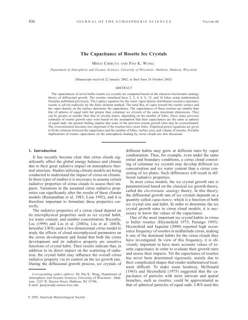
836 JOURNAL OF THE ATMOSPHERIC SCIENCES 

VOLUME 60 

The Capacitance of Rosette Ice Crystals 

MIHAI CHIRUTA AND PAO K. WANG 

Department of Atmospheric and Oceanic Sciences, University of Wisconsin—Madison, Madison, Wisconsin 

(Manuscript received 22 January 2002, in final form 24 October 2002) 

ABSTRACT 

The capacitances of seven bullet rosette ice crystals are computed based on the classical electrostatic analogy 

theory of diffusional growth. The rosettes simulated have 2, 3, 4, 6, 8, 12, and 16 lobes using mathematical 

formulas published previously. The Laplace equation for the water vapor density distribution around a stationary 

rosette is solved explicitly by the finite element method. The total flux of vapor toward the rosette surface and 

the vapor density on the surface determine the capacitance. The capacitances of these rosettes are smaller than 

that of spheres of equal radii but greater than columnar ice crystals of the same maximum dimensions. They 

can be greater or smaller than that of circular plates, depending on the number of lobes. Since many previous 

estimates of rosette growth rates were based on the assumption that their capacitances are the same as spheres 

of equal radii, the present finding implies that some of the previous rosette growth rates may be overestimated. 

The overestimation becomes less important if the rosettes have more lobes. Empirical power equations are given 

to fit the relations between the capacitance and the number of lobes, surface area, and volume of rosettes. Possible 

implications of rosette capacitance on the atmospheric heating by cirrus clouds are also discussed. 

1. Introduction 

It has recently become clear that cirrus clouds significantly 

affect the global energy balance and climate 

due to their great radiative impact on atmospheric thermal 

structure. Studies utilizing climate models are being 

conducted to understand the impact of cirrus on climate. 

In these types of studies it is necessary to assume certain 

radiative properties of cirrus clouds to assess their impacts. 

Variations in the assumed cirrus radiative properties 

can significantly alter the results of these climate 

models (Ramanathan et al. 1983; Liou 1992), and it is 

therefore important to formulate these properties correctly. 

The radiative properties of a cirrus cloud depend on 

its microphysical properties such as ice crystal habit, 

ice water content, and number concentration. Recently, 

Liu (1999) and Liu et al. (2003a; Liu et al. 2003b, 

hereafter LWS) used a two-dimensional cirrus model to 

study the effects of cloud microphysical parameters on 

the cirrus development and found that both the cirrus 

development and its radiative property are sensitive 

functions of crystal habit. Their results indicate that, in 

addition to its direct impact on the scattering of radiation, 

the crystal habit may influence the overall cirrus 

radiative property via its control on the ice growth rate. 

During the diffusional growth process, ice crystals of 

Corresponding author address: Dr. Pao K. Wang, Department of 

Atmospheric and Oceanic Sciences, University of Wisconsin—Madison, 

1225 W. Dayton Street, Madison, WI 53706. 

E-mail: pao@windy.meteor.wisc.edu 

different habits may grow at different rates by vapor 

condensation. Thus, for example, even under the same 

initial and boundary conditions, a cirrus cloud consisting 

of columnar ice crystals may develop different ice 

concentration and ice water content than a cirrus consisting 

of ice plates. Such differences will result in different 

radiative properties. 

In most cirrus models, the ice crystal growth rate is 

parameterized based on the classical ice growth theory, 

called the electrostatic analogy theory. In this theory, 

the diffusional growth rate of ice crystals depends on a 

quantity called capacitance, which is a function of both 

ice crystal size and habit. In order to determine the ice 

crystal growth rates in cirrus cloud models, it is necessary 

to know the values of the capacitance. 

One of the most important ice crystal habits in cirrus 

is bullet rosettes (Heymsfield 1975; Parungo 1995). 

Heymsfield and Iaquinta (2000) reported high occurrence 

frequency of rosettes in midlatitude cirrus, making 

it one of the dominant habits for the cirrus clouds they 

have investigated. In view of this frequency, it is obviously 

important to have more accurate values of rosette 

capacitance in order to evaluate their growth rates 

and assess their impacts. Yet the capacitance of rosettes 

has never been determined rigorously, mainly due to 

their complicated shapes that render mathematical treatment 

difficult. To make some headway, McDonald 

(1963) and Heymsfield (1975) suggested that the capacitance 

of particles with more intricate and spatial 

branches, such as rosettes, could be approximated as 

that of spherical particles of equal radii. LWS used this 

2003 American Meteorological Society

15 MARCH 2003 CHIRUTA AND WANG 

837 

approximation to determine the growth rate of rosettes 

and showed that a cirrus cloud consisting of bullet rosettes 

would have much larger radiative effect than cirrus 

clouds of other ice crystal habits. Given the same 

initial environmental conditions, a peak heating rate due 

to infrared radiation for rosette cirrus, for cirrus ice 

columns and ice plates, and for spheres would be 2.5, 

2, and 6 times greater, respectively. Its heating rate due 

to shortwave solar radiation is also substantially greater 

than other habits. Such a high potential impact on the 

atmospheric heating rates makes the determination of 

the bullet rosette capacitance even more urgent. 

This paper is devoted to the task of calculating the 

capacitance of bullet rosette ice crystals. In the following 

sections, we will first review briefly the electrostatic 

analogy theory of ice crystal diffusional growth to clarify 

the role of the capacitance. Then we will describe 

the techniques of simulating the shapes of these rosettes 

and the methods of determining their capacitance. This 

will be followed by the discussion of the results and 

conclusions. 

2. A brief review of the electrostatic analogy 

theory of ice crystal growth 

The classical theory of ice crystal growth is called 

electrostatic analogy because it dwells on the similarity 

between the equations governing the water vapor distribution 

around an ice crystal and the electrostatic potential 

distribution around an electric conductor of the 

same shape as the ice crystal. A detailed discussion can 

be found in standard textbooks of cloud physics (e.g., 

Pruppacher and Klett 1997; Hobbs 1976; Young 1993). 

The following is a brief outline. 

Note that the electrostatic analogy is only relevant to 

the growth of stationary ice crystals. Another important 

effect on the crystal growth, the ventilation effect that 

results from the motion of the crystal, requires the solutions 

of the Navier–Stokes equations for flow past 

rosette crystals, but unfortunately the solutions are not 

available at present. 

The distribution of water vapor density around a 

stationary ice crystal of arbitrary shape satisfies the Laplace 

equation 

2 

0, 

(1) 

with the following boundary conditions: 

s 

at the crystal’s surface, 

 

 

(2) 

far away from the crystal, 

 

where both s and are constant. In electrostatics, the 

electric potential around a conductor of the same (arbitrary) 

shape as the ice crystal would also satisfies the 

Laplace equation 

2 

0, (3) 

with the boundary conditions 

U on the crystal’s surface, 

 

 

(4) 

0 at the outer boundary of the domain. 

Obviously, equation set (1) and (2) are completely 

equivalent to equation set (3) and (4), the only difference 

being the symbols. Thus, if the set (3) and (4) can be 

solved, the same solution would also satisfy the set (1) 

and (2). However, due to the complicated shapes of most 

ice crystals, we rarely solve these equations directly to 

determine the distributions of and (although this 

was done in Ji and Wang 1999). Instead, since the main 

purpose of such calculations is to determine the ice crystal 

diffusional growth rate given by the integral 

dm D · ds, (5) 

dt 

s 

where m is the mass of the ice crystal, D the diffusivity 

of water vapor in air, and ds the infinitesimal increment 

of an arbitrary surface enclosing the ice crystal, it turns 

out that we can bypass the determination the explicit 

distribution. This understanding stems from the wellknown 

Gauss law in the classical electrostatics, which 

states that the enclosing surface integral of the electric 

flux density equals the total charge Q on the conductor. 

On the other hand, the total charge Q is related to 

the electric potential by the following expression: 

Q C(U 0) CU, (6) 

where C is the capacitance of the conductor. Equation 

(6) is independent of the shape of the conductor. According 

to this analogy (see Pruppacher and Klett 1997 

for details), the term dm/dt in (5) is analogous to Q and 

thus can be calculated by 

dm 4D C( s ). (7) 

dt 

Equation (7) indicates that the growth rate of the ice 

crystal can be determined if its capacitance C is known. 

All other quantities on the right-hand side of (7) are 

independent of the shape. 

The capacitance C in (7) can be either calculated or 

measured experimentally. While the capacitances of some 

simpler ice crystal shapes such as columns and plates 

have been theoretically calculated approximately or measured 

directly by using metal models of the crystals 

(McDonald 1963; Podzimek 1966; also see Pruppacher 

and Klett 1997, chapter 13), neither has ever been attempted 

for the important case of bullet rosettes. To our 

knowledge, the present study is the first to do so. 

3. Mathematical determination of capacitance 

a. Nondimensionalization of the governing equations 

The main idea of determining the capacitance of a 

rosette is to utilize Eq. (7), namely, we shall determine 

dm/dt explicitly and then use (7) to obtain the capacitance 

C. This is analogous to determining the electric


VOLUME 60 

capacitance of a conductor with known potentials on 

the surface and at infinity. To determine dm/dt, we need 

to explicitly solve the water vapor density distribution 

first. The governing equations for our problem are therefore 

Eq. (1), subject to appropriate boundary conditions. 

The Laplace equation will be made dimensionless first 

for the convenience of analysis: 

2 

0, 

(8) 

where the primed quantity in the integrand are nondimensionalized 

according to the following relations: 

 

 

r 

 

, r , (9) 

 

a 

s 

 

where a is the radius of the ice crystal and r the radial 

distance from the origin, which is defined at the center 

of the ice crystal in the present study. The radius of the 

rosette considered here is defined as the distance from 

the center of the rosette to the tip of one of the lobes. 

We assume that all lobes have the same length in this 

study. 

Once the vapor density distribution is determined, 

the capacitance is obtained by 

 

a 

C · ds. (10) 

4 

s 

Smythe (1956, 1962) and Wang et al. (1985) performed 

similar calculations to determine the capacitance of right 

circular cylinders of finite lengths by solving the Laplace 

equation analytically. In view of the more complicated 

rosette shape in the present study, we will use 

numerical techniques instead. 

We need to carefully define appropriate boundary 

conditions for our numerical problem. Since the capacitance 

is a function of the position of these boundaries, 

the capacitance of an isolated conductor will be different 

from the same conductor when it is placed near another 

charged body with a certain potential. This means that 

the distance of the outer boundary may have an effect 

on the precise value of the capacitance. In atmospheric 

clouds, the mean distance between individual cloud particles 

is rather large relative to the particle size, typically 

on the order of many tens to hundreds of particle radii 

(Prupppacher and Klett 1997). Thus the ice particles can 

often be considered as isolated individual particles, and 

hence the most relevant capacitance for our purpose here 

will be that of an isolated ice crystal; that is, the outer 

boundary should be placed at infinity. Thus boundary 

condition (2) is appropriate. In numerical calculations, 

the term ‘‘infinity’’ is replaced by ‘‘sufficiently far 

away.’’ In nondimensional form, the appropriate boundary 

conditions for the present situation are 

 

 

1 on the surface of the rosette, 

0 at a distance far away from the rosette. 

(11) 

b. Treatment of the boundary conditions 

1) THE INNER BOUNDARY 

We will use the finite element techniques to solve the 

Laplace equation (8) subject to the boundary conditions 

(11). This requires setting up a grid system for the computational 

domain between the inner and outer boundaries. 

The first step for this analysis is to prescribe the 

boundary points. 

The inner boundary is the surface of the bullet rosette. 

The shape of a bullet rosette is highly complicated, and 

it is not easy to determine the coordinates of the boundary 

surface. To simplify this problem, we use the successive 

modification of simple shapes (SMOSS) technique 

developed by Wang (1997, 1999, 2002) to simulate 

the shape of ice crystals. The mathematical expression 

specific for this case is given in Wang (1999): 

2 2 

r {[cos (m)] } {[sin (n)] } . 

(12) 

This equation is expressed in spherical coordinates so 

that r is the radial, the zenithal, and the azimuthal 

coordinates. The parameters , , , , , , , and 

are freely adjustable in order to fit the shape of a 

particular rosette. The shape generated by this expression 

will have 2mn lobes or branches. For example, a 

four-branch combination of bullets can be generated by 

the following expression: 

4 20 4 20 

r [1 cos(2) ] [1 sin() ] , (13) 

where m 2 and n 1 here. The width of the branch 

is controlled by and in (12). Obviously, it is impossible 

that such a simple expression will reproduce 

all the intricate structures, but at least it captures the 

essential multilobe feature that is characteristic of bullet 

rosette crystals. 

2) THE OUTER BOUNDARY 

Although the inner boundary of the problem is not 

spherically symmetric, the outer boundary of the present 

problem, if set at infinity, will be a sphere, as the distribution 

of any field whose source is finite (such as the 

rosette considered here) will become spherically symmetric 

when the distance approaches infinity. However, 

in numerical calculations, the distance of the outer 

boundary from the origin has to remain finite and hence 

the field distribution here may deviate from being truly 

spherically symmetric. In the present study, we assume 

that this finite outer boundary surface is also spherical. 

In order to assess the impact of this assumption on the 

accuracy of the results, we performed tests to determine 

how sensitive the results are to the outer boundary distance. 

It turns out that the results are not very sensitive 

to the outer boundary distance as long as it is at least 

seven radii away from the center of the crystal. Further


839 

FIG. 1. The seven simulated bullet rosette ice crystals and their generating equations, surface area (S), volume (V), and the projected 

areas in x, y, and z direction. The areas are in units of a 2 , and the volume in a 3 . 

discussion on the sensitivity tests will be included in 

the next section. 

A brief description of the discretization techniques 

used for the present study and an example of the grid 

structure are given in the appendix. 

4. Results and discussion 

The capacitances of seven bullets rosette crystals are 

calculated using the techniques outlined in the previous 

section. These rosettes have 2, 3, 4, 6, 8, 12, and 16 

lobes. These rosette cases are chosen because their geometrical 

symmetries render them easier for mathematical 

treatment. The mathematical expressions for the 

rosettes and plots of their shapes are shown in Fig. 1. 

The rosettes look visually reasonable when compared 

with photographs of actual samples. More quantitative 

discussions of their geometrical properties are given in 

the next section. Due to the limitation of the formulas, 

it is sometimes difficult to obtain a completely symmetric 

shape for individual lobes. Thus sometimes the 

dimension of a lobe in direction is substantially different 

than that in direction. But the multilobe characteristic 

of the rosettes is well reproduced. The crystals 

generated in this way have the lobes of equal length a. 

Also included in Fig. 1 are values of the rosettes’ total 

surface areas, volumes, and the cross-sectional areas S x , 

S y , and S z projected in the x, y, and z axis, respectively. 

As an example, Fig. 2 shows plots of the projected crosssectional 

areas of an eight-lobed rosette. 

a. Geometrical properties of the modeled rosettes 

It is useful to briefly mention some geometrical properties 

of the modeled rosettes. Figure 3 shows the variation 

of the rosettes’ surface areas and volumes with


VOLUME 60 

FIG. 2. The projected areas S x , S y , and S z of an eight-lobed bullet 

rosette simulated in the study. 

the number of lobes. It appears that while both the surface 

area and volume increase with the number of lobes, 

the increasing rates are not uniform that may be due to 

the specific set of parameter values used. The solid 

curves represent power fit by the following formulas: 

0.7727 2 

A 1.5528N a (surface area) and 

FIG. 4. Variation of surface area vs radius of rosettes. Here N 

represents the number of lobes of the rosette. The thick curve is for 

spheres. 

0.5206 3 

V 0.3257N a (volume). (14) 

Higher-order polynomials can fit even closer, but we 

feel it is unnecessary. 

Figures 4 and 5 show the plots of the surface area 

and volume versus the radius as computed from (14) 

for all seven-rosette cases. It is seen that the surface 

areas of all rosettes, except the 16-lobed ones, are smaller 

than that of a sphere of equal radius. On the other 

hand, the sphere volume is always greater than the volume 

of a rosette regardless of the number of lobes. 

Naturally, as the number of rosette lobes increases, the 

volume increases also. 

Heymsfield and Iaquinta (2000) presented some observational 

results of bullet rosettes in cirrus clouds, and 

it is useful to compare their geometrical properties with 

the simulated models in this study. Since the models 

used in this study are dimensionless, the most convenient 

parameter for comparing the geometrical properties 

is the aspect ratio, defined as the width w divided 

by the length L of a bullet. 

To determine the aspect ratio of the seven rosettes we 

used the maximum width of the lobe as the width of 

the bullet. The length L is of course equal to a of the 

lobe. The aspect ratios of the modeled rosettes, so determined, 

vary between 0.35 0.6. Those with fewer 

lobes are usually associated with larger aspect ratios and 

those with more lobes are associated with smaller aspect 

ratios, but the relation is not monotonic. This range of 

aspect ratios appears to be consistent with the majority 

of the bullet rosettes observed by Heymsfield and Iaquinta 

(2000). 

FIG. 3. Variation of the surface area and volume of the simulated 

rosettes as a function of number of lobes. 

FIG. 5. Variation of volume vs radius of rosettes. Here N represents 

the number of lobes of the rosette. The thick curve is for spheres.


841 

The volume of a bullet rosette calculated using (14) 

is also generally consistent with that calculated using 

the empirical formula given by Heymsfield and Iaquinta. 

For example, the volume of a five-lobed rosette calculated 

from (14) will be the same (0.75 a 3 ) as that 

calculated using their Eq. (A10) if the aspect ratio is 

taken to be 0.45. It is noted that (14) does not include 

the aspect ratio effect, hence the volume calculated by 

it will be different from Heymsfield and Iaquinta’s formula 

if the aspect ratio changes. 

Yang et al. (2000) also suggested a few empirical 

parameters to characterize the geometrical properties of 

nonspherical ice particles including rosettes. Their main 

purpose was for the parameterization of scattering and 

absorption properties of these particles. One of the parameters 

they suggested is the equivalent radius d e defined 

as 1.5 (V/A), where V is the volume and A the 

projected area. The four-and six-lobed rosettes modeled 

in the present study resemble that described in Yang et 

al. (2000) and have d e varying with a in a similar manner, 

but the values are larger for the same maximum 

dimension. The differences are smaller when rosettes 

are small but become much larger when rosettes reach 

millimeter size. More research is needed to understand 

the significance of such differences. 

FIG. 6. The computed capacitance of an eight-lobed rosette as a 

function of the outer boundary distance. 

b. Capacitances of rosettes 

Since both the grid resolution and the distance of 

outer boundary may influence the precision of the results, 

we performed several sensitivity tests in order to 

ensure the accuracy of the computed capacitances. The 

first test is on the sensitivity of grid resolution. Several 

grids were set up for the solutions of in (8) and the 

results compared. If the results are similar (less than 

about 5% difference), the one with the least resolution 

is adopted as the grid for the calculations to achieve 

computational efficiency. 

The second test is on the sensitivity of the distance 

of the outer boundary. This distance was set at different 

values from 2.5 to 15 and the respective capacitance 

was computed accordingly. As an example, the computed 

capacitances of an eight-lobed rosette with different 

outer boundary distances are shown in Fig. 6. We 

see in Fig. 6 that as the distance of the outer boundary 

b increases, the capacitance of the rosette decreases and 

approaches an asymptotic value. This asymptotic value 

should represent the capacitance of an isolated rosette 

(i.e., when the outer boundary is set at infinity) and is 

the value reported here. As mentioned before, the capacitance 

becomes more or less constant for outer 

boundary distance greater than 6 radii. 

To determine the capacitance, the numerical solutions 

of are fed into Eq. (10) and the integral is computed 

numerically. In an exact analytical theory, the results of 

integration is independent of the surface chosen because 

of the steady-state condition implied in the formulation, 

but in numerical calculations these results may be somewhat 

different due to numerical errors in the solutions 

of . In order to ensure accuracy, we performed the 

integration in (10) over 10 different surfaces to make 

sure that errors are insignificant. It turned out that the 

differences are typically less than 5%, thus an averaged 

value of all of these results should be representative of 

the true value of the capacitance. 

The computed capacitances of the rosettes as a function 

of the number of lobes are shown in Fig. 7. The 

slight scatter in the results is largely due to the shape 

parameters chosen in Eq. (12). However, the general 

trend of the curve is fairly clear and the scatter should 

not influence the conclusions to any significant extent. 

It is seen in Fig. 7 that the rosette capacitance increases 

from about 0.5 to near 0.9 (in unit of a) as the number 

of lobes increases from 2 to 16. The capacitance of a 

conducting sphere is its radius a. Thus it appears that the 

capacitance of a rosette will approach that of a sphere if 

the number of lobes approaches infinity, that is, as its 

shape approaches a sphere. The following power relation 

can fit the rosette capacitance curve in Fig. 7: 

0.257 

C 0.434N , (15) 

where C is the capacitance in unit of a and N is the 

number of lobes. 

Figure 7 thus shows that the capacitance of a rosette 

is smaller than that of a sphere of equal radius. This 

implies that calculations of the rosette growth rate based 

on the spherical capacitance assumption overestimate. 

The overestimation is the most serious for rosettes with 

fewer lobes but becomes less if the number of lobes is 

large. 

The capacitances of a thin circular plate and two cases 

of prolate spheroids are also shown in Fig. 7 for comparison. 

These shapes have been used previously as ap-


VOLUME 60 

FIG. 7. Computed capacitance (diamonds) of rosettes as a function 

of number of lobes. Thick solid curve represent power fit by Eq. 

(15). Also shown are the capacitances of a sphere (thin solid line), 

a circular plate (dashed), and two prolate spheroids with semiaxis 

ratio a/b 2 and 5, respectively. The rosettes, the sphere, and circular 

plate all have a radius a. 

proximations for ice plates and ice columns and their 

capacitance formulas are given as 

2a 

C (circular plate) and 

 

2 2 

a c 

C (prolate spheroid), (16) 

ln(2a/c) 

where a and c in the second equation represent the semimajor 

and semiminor axes of the prolate spheroid, respectively 

(see Pruppacher and Klett 1997, chapter 13, 

p. 548). Note that the semilength (the longer dimension) 

instead of the radius of the prolate spheroid is denoted 

as a. McDonald (1963) and Podzimek (1966) performed 

laboratory measurements of the capacitances of metal 

models of ice columns, plates, and dendrites, and their 

results are close to that given by Eq. (16), usually to 

about 10% or less. Only the highly skeleton stellar crystal 

[P1d in Magono–Lee classification, see Magono and 

Lee (1966)] has a capacitance about 23% less than that 

given by the plate in (16). Hence the capacitances given 

by (16) are fairly representative of the atmospheric ice 

crystals. 

We will use the capacitance of a prolate spheroid to 

approximate that of a hexagonal column in the following 

discussion. We see that the capacitance of a two-lobed 

rosette crystal is smaller than that of a short column (a 

2c) (C 0.65) but is greater than that of a long thin 

column (a 5c). A five-lobed rosette has a capacitance 

close to that of a short column. This implies that the 

growth rate of a rosette ice crystal is usually greater 

FIG. 8. Variation of capacitance with radius of rosettes calculated 

using (15). Here N represents the number of lobes of the rosette. The 

thick curve is for spheres. 

than that of a long thin column and may even be greater 

than a short column if it has more than five lobes. 

The capacitance of a circular plate is greater than that 

of rosettes of the same radii up to five lobes, but becomes 

smaller than rosette capacitance as the number 

of rosette lobes increases. If the rosette has more than 

five lobes, its growth rate will be faster than an ice plate 

of the same dimension. 

Figure 8 shows the plot of capacitance versus radius 

for rosettes as computed using (15). The case of spheres 

is also given here for comparison. 

Since the surface area and volume of a rosette are 

important geometrical properties, it is useful to examine 

the relations between the capacitance and these two geometrical 

quantities. Figures 9 and 10 show the variation 

of the capacitance with rosette surface area and volume. 

The capacitance of the rosettes generally increases with 

increasing surface area and volume. The curves represent 

the power fits 

0.3476 

C 0.3636S (surface area) and 

0.4401 

C 0.7472V (volume). (17) 

It is of interest to compare the capacitances between 

rosettes and spheres of equal areas and volumes. To do 

so, we used (14) to calculate the areas and volumes of 

the rosettes and (15) to calculate the capacitances for a 

given N. Figure 11 shows the comparison for equal 

areas. It is seen that rosettes have capacitances larger 

than a sphere of equal area if the number of lobes is 

smaller than 6. For a rosette with more than six lobes, 

the capacitance becomes smaller than that of a sphere 

of equal area, and the more lobes it has, the smaller the 

capacitance becomes. One factor that contributes to this


843 

FIG. 9. Computed rosette capacitance (squares) as a function of rosette 

surface area. The solid curve represents power fit by Eq. (17). 

FIG. 11. Variation of capacitance with rosette surface area. Here 

N represents the number of lobes of the rosette. The thick curve is 

for spheres. 

behavior is the linear dimension of rosettes. A rosette 

with few lobes needs to be substantially longer than a 

sphere in order to have same area. Such a long rosette 

tends to have higher capacitance than the sphere. On 

the other hand, a rosette with more lobes need not be 

much longer than a sphere to have the same area. Figure 

4 shows that, as the number of lobes increases the rosettes 

modeled here, the surface area of a rosette becomes 

closer to that of a sphere of equal radius. A rosette 

with 16 lobes even has an area greater than a sphere of 

equal radius. Of course, the linear dimension is not the 

only factor deciding the capacitance and other factors 

should be considered to fully understand the behavior 

of the curves in Fig. 11. 

The comparison for equal volume is given in Fig. 12, 

which shows that the capacitances of rosettes are greater 

than a sphere of equal volume in all cases, and the more 

the lobes, the greater the capacitance. More studies are 

being conducted to understand this phenomenon. 

Since equal volume means equal amount of water 

content, Fig. 12 implies that, given the same amount of 

water substance and holding other environmental conditions 

constant, a cirrus cloud composed of bullet ro- 

FIG. 10. Computed rosette capacitance (squares) as a function of 

rosette volume. The solid curve represents power fit by Eq. (17). 

FIG. 12. Variation of capacitance with rosette volume. Here N represents 

the number of lobes of the rosette. The thick curve is for 

spheres.


VOLUME 60 

settes will grow more vigorously than one composed of 

spheres (e.g., frozen drops). In addition, the more lobes 

the rosettes have, the faster they will grow. Such rapid 

growth rates would imply greater impact on the cloud 

heating of the atmosphere. This is one of the main conclusions 

of LWS’s study and suggests that the impact 

of ice habit, especially that of rosettes, on the cirrus 

development has to be assessed carefully. 

Finally, it is known that rosettes can consist of hollow 

bullets, which are not represented by Eq. (12) and whose 

capacitances may differ from that given above. More 

research is needed to determine the capacitance of such 

hollow rosettes. 

5. Conclusions 

Heymsfield and Platt (1984), Heymsfield and Mc- 

Farquhar (1996, 2002), McFarquhar and Heymsfield 

(1996), and Heymsfield and Iaquinta (2000) indicated 

that ice columns and bullet rosettes dominate the midlatitude 

cirrus, so it is meaningful to compare the capacitances 

of these two ice habits. The results presented 

above show that those rosettes with five lobes have capacitances 

closer to that of ice columns of similar maximum 

dimensions, but those with more lobes would 

have capacitances much greater than columns. The rosette 

capacitances, even those with few lobes, are greater 

than long, thin columns. Since the growth rate is directly 

proportional to the capacitance, this implies that rosettes 

will, in general, grow much faster than columns. On the 

other hand, the assumption that a rosette will have capacitance 

of a sphere of equal radius would overestimate 

the growth rate. The magnitude of overestimation would 

depend on the number of lobes of the rosette in question. 

Observations suggest that the dominant number of 

rosette lobes is either about 3 4 (Kikuchi 1968) or 5 

(Heymsfield and Iaquinta 2000; A.J. Heymsfield 2001, 

personal communication). In either case, the capacitance 

of rosettes will definitely be greater than the columns 

(more than 2 times larger than the long thin columns) 

but smaller than the spheres of the same maximum dimensions. 

Since the growth rate is directly proportional 

to the capacitance, an accurate assessment of the rosette 

growth rate in a particular cirrus cloud seems to hinge 

upon a good estimate of their mean number of lobes. 

The rosette growth rate estimates based on the new 

capacitance results will certainly impact on the development 

of cirrus clouds and thence the heating rates of 

the atmosphere caused by the presence of cirrus. But 

due to the complexity in the interaction between cloud 

dynamics and microphysics, we need to use a realistic 

cirrus model to assess these impacts. 

Acknowledgments. We thank A. Heymsfield for information 

about the geometrical properties of the bullet 

rosettes in cirrus. P. Yang and two anonymous reviewers 

also gave helpful comments that result in improvements 

of the paper. This work is supported by the NSF Grant 

ATM-9907761. 

APPENDIX 

Finite Element Techniques Used for the 

Present Study 

This appendix provides a brief summary of the discretization 

technique used for numerically solving the 

Laplace equation for the water vapor density and the 

equations that give the Cartesian components of the water 

vapor flux density. The specific discretization technique 

we used is the finite element analysis and readers 

are referred to standard textbooks for a general discussion 

(see, e.g., Fletcher 1984). Since the discussions of 

finite element methods in most textbooks are confined 

to two-dimensional cases whereas the present application 

is three-dimensional, we feel it is useful to provide 

some details. 

The finite elements chosen for the present study were 

tetrahedrons. We used quadratic functions for the water 

vapor density and linear functions for the flux density 

components for interpolation purpose. This combination 

of interpolation functions ensures a continuous water 

vapor flux density profile. The water vapor flux density 

continuity allows small numerical errors in the capacitance 

using a reasonable discretization of the analysis 

domain. 

The water vapor density approximation on a tetrahedron 

is given by 

10 

i i 

i1 

ˆ N , (A1) 

where N i s are the quadratic interpolation functions 

(Dawe 1987) and i are the values of the water vapor 

density at the vertices and midpoints of edges of the 

tetrahedron. 

Since ˆ is an approximation of the exact solution, it 

does not satisfy the Laplace equation and hence we have 

a residual R(x, y, z, N i ): 

2 2 2 

ˆ ˆ ˆ 

R(x, y, z, N i). (A2) 

2 2 2 

x y z 

The application of the weighted residual method 

(Fletcher 1984) to minimize the residual term leads to 

the following elemental algebraic equation: 

Ae 

ˆ 0, 

(A3) 

with the components of the A e matrix being 

Ni Nj Ni Nj Ni N 

e 

j 

Aij ˆ j 

 

 

dV, (A4) 

x x y y z z 

V e 

where the integral is calculated over the volume of the 

finite element. 

The elemental equations are assembled over the 

whole analysis domain in accordance with the topology


845 

of the discretization. This forms an algebraic system of 

equations whose solutions are the values of the water 

vapor density at the nodes of the discretization. 

The approximate value of the x component of water 

vapor flux density in polynomial form is given by 

4 

x i xi 

i1 

ĵ Lj , (A5) 

where L i s are the linear interpolation functions given in 

Dawe (1987) and j xi s are the values of the x component 

of vapor density flux in the tetrahedron vertices. 

Using the approximate value of the water vapor density 

ˆ , the x component of vapor flux density can be 

written as 

1 ˆ ĵ 

 

x . (A6) 

D x 

Using the weighted residual method described previously, 

we obtain the elemental equations for the x 

component of vapor flux density 

e e 

e 

B ĵx f x , 

(A7) 

where the components of the matrix B e are 

e 

Bij LiLj 

dV, (A8) 

V e 

and those of the matrix fe 

x are 

10 

1 N 

e 

j 

f xi Li ˆ j 

 

dV. (A9) 

D 

j1 x 

V e 

Assembling the elemental equations (A7) over the 

whole domain, we again obtain a system of algebraic 

FIG. A1. The discretization into finite elements of the analysis 

domain for an eight-lobed bullet rosette ice crystal. The length of a 

lobe is a and the radius of the outer sphere is b 5 a. 

equations whose solutions are the x component values 

of vapor flux density at the nodes of the discretization. 

The y and z components of vapor flux density are obtained 

in a similar fashion. 

In the initial formulation as described in section 2, 

the inner boundary of the domain is the rosette surface 

and the outer boundary is a sphere with radius b, centered 

at the center of the crystal. In actual calculations 

we only need to use a portion of this domain because 

of the symmetry of the rosettes. However, this results 

in new boundary surfaces when we cut the original domain 

into separate portions (see Fig. A1). It is therefore 

necessary to specify the conditions in these new surfaces. 

Here we use the requirement that the normal derivative 

of the water vapor density be zero as the boundary 

conditions. 

REFERENCES 

Dawe, D. J., 1987: Curved beam and arch elements. Finite Element 

Handbook, H. Kardestuncer, Ed., McGraw-Hill, 2.128–2.129. 

Fletcher, C. A. J., 1984: Computational Galerkin Methods. Springer, 

300 pp. 

Heymsfield, A. J., 1975: Cirrus uncinus generating cells and the evolution 

of cirroform clouds. III. J. Atmos. Sci., 32, 799–808. 

——, and C. M. R. Platt, 1984: A parameterization of the particle 

size spectrum of ice clouds in terms of the ambient temperature 

and ice water content. J. Atmos. Sci., 41, 846–855. 

——, and G. M. McFarquhar, 1996: High albedos of cirrus in the 

tropical Pacific warm pool: Microphysical interpretations from 

CEPEX and from Kwajalein, Marshall Islands. J. Atmos. Sci., 

53, 2424–2451. 

——, and J. Iaquinta, 2000: Cirrus crystal terminal velocities. J. 

Atmos. Sci., 57, 914–936. 

——, and G. M. McFarquhar, 2002: Mid-latitude and tropical cirrus 

microphysical properties. Cirrus. D. Lynch, Ed., Oxford University 

Press, 288 pp. 

Hobbs, P. V., 1976: Ice Physics. Oxford University Press, 837 pp. 

Ji, W., and P. K. Wang, 1999: Ventilation coefficients of falling ice 

crystals at low–intermediate Reynolds numbers. J. Atmos. Sci., 

56, 829–836. 

Kikuchi, K., 1968: On snow crystals of bullet type. J. Meteor. Soc. 

Japan, 46, 128–132. 

Liou, K. N., 1992: Radiation and Cloud Processes in the Atmosphere. 

Oxford University Press, 487 pp. 

Liu, H. C., 1999: A numerical study of cirrus clouds. Ph.D. thesis, 

Dept. of Atmospheric and Oceanic Sciences, University of Wisconsin—Madison, 

257 pp. 

——, P. K. Wang, and R. E. Schlesinger, 2003a: A numerical study 

of cirrus clouds. Part I: Model description. J. Atmos. Sci., in 

press. 

——, ——, and ——, 2003b: A numerical study of cirrus clouds. 

Part II: Effects of ambient temperature, stability, radiation, ice 

microphysics and microdynamics on cirrus evolution. J. Atmos. 

Sci., in press. 

Magono, C., and C. W. Lee, 1966: Meteorological classification of 

natural snow crystals. J. Fac. Sci. Hokkaido University, Ser. VII, 

2, 321–335. 

McDonald, J. E., 1963: Use of electrostatic analogy in studies of ice 

crystal growth. Z. Angew. Math. Phys., 14, 610. 

McFarquhar, G. M., and A. Heymsfield, 1996: Microphysical characteristics 

of three anvils sampled during the Central Equatorial 

Pacific Experiment. J. Atmos. Sci., 53, 2401–2423. 

Parungo, F., 1995: Ice crystals in high clouds and contrails. Atmos. 

Res., 38, 249–262.


VOLUME 60 

Podzimek, J., 1966: Experimental determination of the ‘‘capacity’’ 

of ice crystals. Studia Geophys. Geodet., 10, 235–238. 

Pruppacher, H. R., and J. D. Klett, 1997: Microphysics of Clouds and 

Precipitation. Kluwer Academic, 954 pp. 

Ramanathan, V., E. J. Pitcher, R. C. Malone, and M. L. Blackmon, 

1983: The response of a spectral general circulation model 

to refinements in radiative processes. J. Atmos. Sci., 40, 605– 

630. 

Smythe, W. R., 1956: Charged right circular cylinders. J. Appl. Phys., 

27, 917–920. 

——, 1962: Charged right circular cylinders. J. Appl. Phys., 33, 2966– 

2967. 

Wang, P. K., 1997: Characterization of ice particles in clouds by 

simple mathematical expressions based on successive modification 

of simple shapes. J. Atmos. Sci., 54, 2035–2041. 

——, 1999: Three-dimensional representations of hexagonal ice crystals 

and hail particles of elliptical cross sections. J. Atmos. Sci., 

56, 1089–1093. 

——, 2002: Ice Microdynamics. Academic Press, 273 pp. 

——, C. H. Chuang, and N. L. Miller, 1985: Electrostatic, thermal 

and vapor density fields surrounding stationary columnar ice 

crystals. J. Atmos. Sci., 42, 2371–2379. 

Yang, P., K. N. Liou, K. Wyser, and D. Mitchell, 2000: Parameterization 

of the scattering and absorption properties of individual 

ice crystals. J. Geophys. Res., 105, 4699–4718. 

Young, K. C., 1993: Microphysical Processes in Clouds. Oxford University 

Press, 427 pp.

The Capacitance of Rosette Ice Crystals - University of Wisconsin ...

Create successful ePaper yourself

Delete template?

Save as template?