Vectors and Tensors R. Shankar Subramanian - Noppa

2005
Vectors and Tensors
R. Shankar Subramanian
Good Sources
R. Aris, Vectors, Tensors, and the Equations of Fluid Mechanics, Prentice Hall (1962).
and Appendices in
(i) R. B. Bird, W. E. Stewart, and E. N. Lightfoot, Transport Phenomena, John Wiley, 2002.
(ii) J. Slattery, Momentum, Energy, and Mass Transfer in Continua, McGraw-Hill, 1972.
Some Basics
We encounter physical entities such as position, velocity, momentum, stress, temperature heat flux,
concentration, and mass flux in transport problems - there is a need to describe them in
mathematical terms and manipulate the representations in various ways. This requires the tools of
tensor analysis.
Scalars
An entity such as temperature or concentration that has a magnitude (and some units that need not
concern us right now), but no sense of direction, is represented by a scalar.
Vectors
In contrast, consider the velocity of a particle or element of fluid; to describe it fully, we need to
specify both its magnitude ( in some suitable units) and its instantaneous spatial direction. Other
examples are momentum, heat flux, and mass flux. These quantities are described by vectors. In
books, vectors are printed in boldface. In ordinary writing, we may represent a vector in different
ways.
vvv , ,
or vi
Gibbs notation
index notation
The last requires comment. Whereas we represent the vectorial quantity with a symbol, we often
know it only via its components in some basis set. Note that the vector as an entity has an invariant
identity independent of the basis set in which we choose to represent it.
1

In index notation, the subscript “i” is a free index - that is, it is allowed to take on any of the three
values 1, 2, 3, in 3-dimensional space. Thus, really stands for the ordered set v , v , v .
Basis Sets
v ( )
i
1 2 3
The most common basis set in three-dimensional space is the orthogonal triad ( i, j,
k )
corresponding to a rectangular Cartesian coordinate system. i stands for a unit vector in the x-
direction and j and k represent unit vectors in the y and z-directions respectively. Note that this is
not a unique basis set. The directions of
i, j,
k depend on our choice of the coordinate directions.
There is no reason for the basis set to be composed of orthogonal vectors. The only requirement is
that the three vectors chosen do not lie in a plane. Orthogonal sets are the most convenient,
however.
We find the components of a vector in the directions of the base vectors by taking inner (dot)
products.
v = v⋅ i, v = v⋅ j,
v = v⋅
k
Then, v = vxi + vy j+
vzk
x y z
You can verify the consistency of the above by taking inner products of both sides of the equation
with the base vectors and recognizing that the base vectors are orthogonal.
i ⋅ j = j⋅ k = k⋅i
≡
0
The order of the vectors in the inner product is unimportant.
a⋅ b = b⋅
a
Scalar and Vector Fields
In practice the temperature, velocity, and concentration in a fluid vary from point to point (and often
with time). Thus, we think of fields - temperature field, velocity field, etc.
In the case of a vector field such as the velocity in a fluid, we need to represent the velocity at every
point in space in the domain of interest. The advantage of the rectangular Cartesian basis set
( i, j,
k) is that it is invariant as we translate the triad to any point in space. That is, not only are
these base vectors of unit length, but they never change direction as we move from one point to
another, once we have chosen our x, y , and z directions.
2

Vector Operations
The entity v has an identity of its own. Its length and spatial direction are independent of the basis
set we choose. As the vectors in the basis set change, the components of v change according to
standard rules.
Vectors can be added; the results are new vectors. If we use component representation, we simply
add each component. Subtraction works in a similar manner.
Vectors also can be multiplied, but there are two ways to do it. We define the dot and cross
products, also known as inner and vector products, respectively, as shown below.
a⋅ b = axbx + ayby + azbz
is a scalar. We commonly use a numerical subscript for the components; in
( )
this case, the basis set is the orthogonal triad e
() , e
1 ( 2) , e
( 3)
. Let
Then,
=
1
+
2
+
3 3
a a e a e a e
() 1 ( 2) ( )
a⋅ b = ab
1 1+ a2b2+
a3b3
3
= ∑ ab
i i
i=
1
In the above, we usually omit
implied.
3
∑
i=1
. When an index is repeated, summation over that index is
a⋅ b = ab
This is called the summation convention
i
i
a⋅ a = aa = a 2 or a
i
i
2
where a is the length of
as the basis set is altered.
a and is invariant; “invariant” means that the entity does not change
a × b is the vector product. As implied by the name, it is a vector; it is normal to the plane
containing a and b . ( a, b,
a× b) form a right-handed system (this is an arbitrary convention , but
we have to choose one or the other, so we choose “right”). The order is important, for,
a× b =− b×
a
3

that is, b× a points opposite to a× b.
We can write
a × b =
e
a
b
(1)
1
1
e
a
b
(2)
2
2
e
a
b
(3)
3
3
There is a compact representation of a determinant that helps us write
a× b = ε ab
ijk i j
(Note that k is a free index. The actual symbol chosen for it is not important; what matters is
that the right side has one free index, making it a vector)
ε
ijk
is called the permutation symbol
ε = 0 if any two of the indices are the same
ijk
=+ 1if i, j,
k
form an even permutation of 1, 2, 3 [example: 1,2,3]
=−1if i, j,
k
We can assign a geometric interpretation to
a and b is θ , then
a⋅ b = a b cos θ
form an odd permutation of 1, 2, 3 [example: 2, 1, 3]
a⋅ b and a× b. If the angle between the two vectors
and the length of a× b is ab sinθ
. You may also recognize absinθ as the area of the
parallelogram formed by a and b as two adjacent sides. Given this, it is straightforward to see that
a⋅ b× c = ε ab c
ijk i j k
is the volume of the parallelepiped with sides ab , ,andc
Second Order Tensors
. This is called the triple scalar product.
Note that we did not define vector division. The closest we come is in the definition of second-order
tensors!
4

Imagine
Instead, we write
a
b =Τ
a
=Τ⋅ b
A tensor (unless explicitly stated otherwise we’ll only be talking about “second-order” and shall
therefore omit saying it every time) “operates” on a vector to yield another vector. It is very useful
to think of tensors as operators as you’ll see later.
Note the “dot” product above. Using ideas from vectors, we can see how the above equation may be
written in index notation.
a
i
=Τijb
j
It is important to note that b ⋅Τ would be biΤ ij
and would be different from
Τ⋅ b in general.
The two underbars in Τ now take on a clear significance; we are referring to a doubly subscripted
entity. We can think of a tensor as a sum of components in the same way as a vector. For this, we
use the following result.
e
⋅Τ⋅ e =Τ Scalar
() i ( j) ij
We’re not using index notation here
Thus, to get
Τ
23
we would find e( )
⋅Τ⋅e
2 ( 3 ). We can then think of T as a sum.
Τ=Τ e e +Τ e e +Τ e e
() 1 () 1 () 1 ( 2) () 1 ( 3)
11 12 13
+Τ e e +Τ e e +Τ e e
( 2) () 1 ( 2) ( 2) ( 2) ( 3)
21 22 23
+Τ e e +Τ e e +Τ e e
( 3) () 1 ( 3) ( 2) ( 3) ( 3)
31 32 33
What are the quantities e
()
e
1 ( 2)
and others like them? They are called dyads. They are a basis set
for representing tensors. Each is a tensor that only has one component in this basis set. Note that
e e ≠ e e .
() i ( j) ( j) ( i)
You can see that tensors and matrices have a lot in common!
5

In fact, we commonly write the components of a tensor as the elements of a 3 x 3 matrix.
⎛Τ Τ Τ
⎜
Τ Τ Τ
⎜
⎝Τ Τ Τ
11 12 13
21 22 23
31 32 33
⎞
⎟
⎟
⎠
Naturally, as we change our basis set, the components of a given tensor will change, but the entity
itself does not change. Of course, unlike vectors, we cannot visualize tensors – we only “know”
them by what they do to vectors that we “feed” them!
A good example of a tensor in fluid mechanics is the stress at a point. To completely specify the
stress vector, we not only need to specify the point, but also the orientation of the area element. At a
given point, we can orient the area in infinitely many directions, and for each orientation, the stress
vector would, in general be different.
Force
Stress =
Area
← has magnitude and direction
← has magnitude and direction
In fact, we can show that stress is indeed a tensor (for proof, see Aris, p. 101). So, we get
t
= n⋅Τ
n
t
The symbol n represents the unit normal (vector) to the area element, and t is the stress vector
acting on that element. The second-order tensor Τ completely describes the state of stress at a
point. By convention, t is the stress exerted by the fluid into which n points on the fluid adjoining
it.
Invariants
Just as a vector has one invariant (its length), a tensor has three invariants. They are defined as
follows.
6

Let A or A
ij
be the tensor.
↓ abbreviation
I = A = tr A = A
A
trace{ } { }
ii
where
1
II ⎡I II
2 ⎣
IIA
2
A
=
A
−
A
{ }
⎤
⎦
= tr A⋅ A Note: A⋅ A is the tensor Aij A
jk
III
A
= Determinant of A = Det{ A}
= ε
A A A
ijk 1i 2 j 3k
= ε
A A A
ijk il j 2 k 3
As the basis set is changed, the invariants do not change even though the components of the
tensor may change. For more details, consult Aris, p. 26, 27 or Slattery, p. 47, 48.
A symmetric tensor
A ij
is one for which A ij
= A . Thus, there are only six independent
components. Stress is a symmetric tensor (except in unusual fluids). Symmetric tensors with real
elements are self-adjoint operators, a concept about which you can learn more in advanced work.
A skew-symmetric tensor
A
ij
is one for which A ij
diagonal elements must be zero ( A A )
ji
= − A . You can see immediately that the
since
ii
=−
ii
. Skew-symmetric tensors have only three
independent components. Vorticity is an example of a skew symmetric tensor.
If we write a skew-symmetric tensor
A
ij
in the form
ji
⎛0
⎜
−a
⎜
⎝a
a
0
3 2
3 1
− a
2 1
− a ⎞
⎟
a
0 ⎟
⎠
We can see that there is a vector a that can be formed using the elements of A
ij
. The two are
related by the following result, which is useful in the context of the physical significance of
vorticity.
7

A⋅ x = x×
a
There is a special tensor that leaves a vector undisturbed. It is called the identity or unit tensor
I .
⎛100⎞
⎜ ⎟
I = 010
⎜001⎟
⎝ ⎠
I ⋅ x = x
for any x
In index notation, we write I as δ
ij
, the Kronecker delta.
Symmetric tensors have a very special property. Remember that we define a tensor at a point; at that
point, there are three special directions, orthogonal to each other, associated with a symmetric
tensor. When the tensor operates on a vector in one of these directions, it returns another vector
pointing in the same (or exactly opposite) direction! The new vector, however, will have a different
length in general. This magnification factor in the length is called the principal value or eigenvalue
of the tensor. It can, of course, be either smaller or larger than one; we call it magnification (for
convenience) in both cases.
Because there are, in general, three directions that are special, there are usually three distinct
principal values, one associated with each direction. Even for tensors that are not symmetric, there
are three principal values; however these need not all be real. Sometimes, two are complex. Even
when the principal values are real, the directions associated with them need not be orthogonal if the
tensor is not symmetric.
The problem for the principal or eigenvalues of A is
Therefore,
A⋅ x = λx ≡λI ⋅ x
⎡
⎣A−λ
I⎤
⎦ ⋅ x = 0
From linear algebra, for non-trivial solutions of the above system to exist, we must have
det ⎡
⎣A− λ I⎤
⎦ = 0
The resulting third degree equation for the eigenvalues is
− λ + I λ − II λ+ III = 0
3 2
A A A
8

and has three roots λ1,
λ2,
and λ
3
. When these roots are each used, in turn, and we solve for x , we
obtain an eigenvector that is known only to within an arbitrary multiplicative constant. Commonly,
the eigenvector is normalized so that it has unit length.
From the above, you can see that corresponding to a symmetric tensor, there is a special rectangular
Cartesian set of basis vectors. If we choose this as the basis set, the tensor will have a simple
diagonal form with the diagonal components being the eigenvalues.
If you’re wondering what happens when two eigenvalues are identical, it is easy to show that any
vector in the plane normal to the third eigenvector (corresponding to the third eigenvalue) is
acceptable as an eigenvector. In other words, on that plane, the tensor operating on a vector in any
direction will yield a vector in the same direction with a magnification factor corresponding to the
repeated eigenvalue.
If all three eigenvalues are identical, then any direction in space will be acceptable as the direction of
the eigenvectors. Such a tensor is called isotropic for this reason. I is an isotropic tensor with
eigenvalues equal to unity. Any scalar multiple of I also is isotropic.
Finally, you probably have already realized that when an eigenvalue is negative, the tensor operating
on an eigenvector in the corresponding direction alters its length appropriately and reverses the
direction.
Vector Calculus
If we consider a scalar field such as temperature, we find the rate of change with distance in some
direction, x , by calculating ∂Τ ∂ x . How can we represent the rate of change in three-dimensional
space without specifying a particular direction? We do this via the gradient operator. The entity
∇Τ [we call it “grad T”] is a vector field. At a given point in space, the vector, ∇Τ , points in the
direction of greatest change of T. To obtain the rate of change of T at that point in any specified
direction, n , we simply “project” ∇Τ in that direction.
∂Τ =∇Τ⋅ n
∂ n
unit vector
Surfaces in space on which a field has the same value everywhere are contours. In the case of
temperature fields, these contours are called isotherms. Along such a surface, the temperature
cannot change. Therefore, the ∇Τ vector is everywhere normal to isothermal surfaces since it must
yield a value of zero when projected onto such surfaces.
It is straightforward to establish from the definition that
9

∂ ∂
∇≡ e + e + e
∂ ∂
() 1 ( 2) ( 3)
∂
∂
x1 x2
x 3
in a rectangular Cartesian coordinate system ( , , )
x x x .
1 2 3
Note that ∇ is an operator and not a vector. So, you should exercise care in manipulating it.
The ∇ operator is the generalization of a derivative. We can differentiate vector fields in more than
one way.
Divergence
∇⋅ v or div v is called the divergence of the vector field v . If the rectangular Cartesian
components of v are vv, v,
then
1, 2 3
∂v
∂v
∂v
1 2 3
∇⋅ v = + +
∂x1 ∂x2
∂x 3
As you can see, the result is a scalar field.
Curl
∇× v or curl v is a vector field. As the name implies, it measures the “rotation” of the vector
v .
Again, in ( x 1,
x 2
, x 3 ) coordinates,
e e e
() 1 ( 2) ( 3)
∂ ∂ ∂
∇× v = ∂ x ∂ x ∂ x
1 2
v v v
1 2
3
3
= ε
ijk
∂v
j
∂x
i
There are two important theorems you should know. They are simply stated here without proof.
10

Divergence Theorem
If the volume V in space is bounded by the surface S ,
∫ ∫
V
∇⋅ adV = dS⋅a
S
dS
V
S
The vector field a should be continuous and differentiable. The symbol dS represents a vector
surface element. If n is the unit normal to the surface,
dS = n dS
The entity dV is a volume element. In the theorem, the left side is a volume integral and the right
side is an integral over the surface that bounds the volume. Finally, a need not be a vector field, but
can be a tensor field of any order.
The divergence theorem, also known as Green’s transformation, is a very useful result that
permits us to convert volume integrals into surface integrals. By applying it to an infinitesimal
volume, you can visualize the physical significance of the divergence of a vector field at a point as
the outward “flow” of the field from that point.
Stokes Theorem
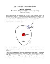
This permits the conversion of integrals over a surface to those around a bounding curve. Imagine a
surface that does not completely enclose a volume, but rather is open, such as a baseball cap. Let S
be the surface and C, the curve that bounds it.
11

t
S
C
If a vector field a is defined everywhere necessary, and is continuous and differentiable, Stokes
theorem states:
S
( )
C
∫ ∫
∇× a ⋅ dS = a⋅t ds
dS : vector area element on S
ds: scalar line element on C
t : unit tangent vector on C
The integral on the right side is known as the circulation of a around the closed curve C. The field
a appearing in the theorem can be replaced by a tensor field of any desired order.
By imagining the surface S to lie completely on the plane of the paper as shown, you can
S
C
visualize the physical significance of
∇× a . If you make S shrink to an infinitesimal area, the area
12

integral on the left side becomes the product of the component of ∇× a normal to the plane of the
paper and the area. The line integral is still the circulation around an infinitesimal closed loop
surrounding the point. If a is the velocity field v , by making the boundary an infinitesimal circle
of radius ε , the right side can be seen to be approximately 2 πε v , where v is the magnitude of the
2
velocity around the loop. The left side is approximately πε (∇ × v)
⋅ n where n is the unit normal to
1
v
the plane of the paper. Therefore, (∇ × v)
⋅n
≈ , which becomes the instantaneous angular
2
ε
velocity of the fluid at the point on the plane of the paper as ε →0
. Because there is nothing unique
1
about the choice of the plane of the paper, we can see that ( ∇ × v)
in fact represents the
2
instantaneous angular velocity vector of a fluid element at a given point, the component of which in
any direction is obtained by projecting in that direction.
The Gradient of a Vector Field
Just as we defined the gradient of a scalar field, it is possible to define the gradient of a vector or
tensor field. If v is a vector field, ∇ v is a second-order tensor field. The rate of change of v in
any direction n is given by
∂ v
∂n
=∇ v ⋅ n
13