Abaqus Technology Brief Automotive Brake Squeal Analysis Using ...

2
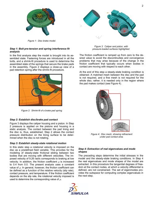
Figure 1: Disc brake model.
Step 1: Bolt pre-tension and spring interference fit
analysis
In the first analysis step the model is brought into its assembled
state. Fastening forces are introduced in all the
bolts, and a shrink-fit procedure is used to determine the
assembled state of the springs that secure the brake pads
in the assembly. Figure 2 displays a close-up view of a
pad retention spring after the shrink-fit procedure.
Figure 3: Caliper and piston, with
pressure-loaded surfaces highlighted.
The friction coefficient is ramped up from zero to the desired
value to avoid the discontinuities and convergence
problems that may arise because of the change in the
friction coefficient that typically occurs when bodies in
contact are moving with respect to each other.
At the end of this step a steady-state braking condition is
obtained. A matched mesh between the disc and the pad
is not required, and a fine mesh is not required for the
whole disc; rather, it is needed only in the region where
the pad makes contact (see Figure 4).
Figure 2: Shrink-fit of a brake pad spring.
Step 2: Establish disc/brake pad contact
Figure 3 displays the caliper housing and a piston. In Step
2 pressure is applied on the pistons and housing in a
static analysis. The contact between the pad lining and
the disc is, thus, established. Step 2 allows the contact
pressure distribution on the lining surface to be determined
when the disc is not rotating.
Step 3: Establish steady-state rotational motion
In this static step a rotational velocity is imposed on the
disc as a predefined field variable. This provides for the
modeling of steady-state frictional sliding between two
bodies that are moving with different velocities. The imposed
velocity of 9.26 rad/s corresponds to braking at low
velocity. In addition, the friction coefficient μ is increased
to 0.4 from 0.0. The present analysis uses a constant
value of μ. In general, however, the friction coefficient can
be defined as a function of the relative velocity (slip rate),
contact pressure, and temperature. If the friction coefficient
depends on the slip rate, the rotational velocity imposed is
used to determine the corresponding value of μ.
Figure 4: Disc mesh, showing refinement
under pad contact area.
Step 4: Extraction of real eigenvalues and mode
shapes
The preceding steps determine the initial stresses in the
model and the steady-state braking conditions. In Step 4
the real eigenvalues and mode shapes of the model are
extracted. In this procedure the tangential degrees of freedom
at the contact nodes, at which a velocity differential is
defined, are not constrained. The set of eigenmodes provides
the subspace for computing complex eigenvalues in
the next step.