Localized Supervised Metric Learning on ... - Researcher - IBM

More documents

Recommendations

Info

epresented by a N-dimensional feature vector x. Examples of features are the mean and variance of the sensor measures, or Wavelet coefficients. The prior belief of physicians is captured as labels on some of the patients. With this formulation, our goal is to learn a generalized Mahalanobis distance between patient x i and patient x j defined as: √ d m (x i , x j ) = (x i − x j ) T P(x i − x j ) (1) where P ∈ R N×N is called the precision matrix. Matrix P is positive semi-definite and is used to incorporate the correlations between different feature dimensions. The key is to learn the optimal P such that the resulting distance metric has the following properties: Figure 1. Retrieving patients based on their clinical similarity to a query patient and using the retrieved patients to project the evolution of patient’s clinical characteristics. comparison. In this paper, we leverage both statistical methods and Wavelet methods to extract features over the temporal data. <strong>Supervised</strong> metric learning has been studied in the past [11, 12, 5]. The goal has been to learn a distance metric such that samples in the same class are close and those in different classes are far away. The common treatment is to add constraints and regularization terms into the objective function and then to solve it using optimization methods. To avoid a large number of constraints, in this paper we model this problem as trace ratio problem which can be solved effectively (similar to Wang et al. [9]). 3 <strong>Localized</strong> <strong>Supervised</strong> <strong>Metric</strong> <strong>Learning</strong> In this section we present the supervised metric learning problem in the context of patient similarity measure. When a physician looks for similar patients in a database, the similarity is often based not only on quantitative measurements such as lab results, sensor measurements, age and sex, but also on the physician’s assessment of the disease type and stage. The assessment would potentially influence the relative importance a physician places on different measurements or groups of measurements. To compute this specific notion of similarity, we propose to learn a distance metric that can automatically adjust the importance of each numeric feature by leveraging the physician’s belief. Formally, quantitative measurements of a patient are • Within-class compactness: patients of the same label are close together; • Between-class scatterness: patients of different labels are far away from each other. To formally measure these properties, we use two kinds of neighborhoods as defined in [10]: The homogeneous neighborhood of x i , denoted as Ni o , is the k-nearest patients of x i with the same label. The heterogeneous neighborhood of x i , denoted as Ni e , is the k-nearest patients of x i with different labels. Based on these two neighborhoods, we define the local compactness of point x i as C i = ∑ d 2 m(x i , x j ) (2) x j∈N o i and the local scatter ness of point x i as S i = ∑ x k ∈N e i d 2 m(x i , x k ) (3) The discriminability of the distance metric d m is defined as ∑ J = ∑ i C ∑ ∑ i i x j∈N (x i i S = o i − x j ) T P(x i − x j ) ∑ ∑ i i x k ∈N (x i e i − x k ) T P(x i − x k ) (4) The goal is to find a P that minimizes J , which is equivalent to minimizing the local compactness and maximizing the local scatterness simultaneously. In contrast with linear discriminant analysis [4] , which seeks for a discriminant subspace in a global sense, the localized supervised metric aims to learn a distance metric with enhanced local discriminability. To minimize J , we formulate the problem as a trace ratio minimization problem [9] and use the decomposed Newtown’s method to find the solution [6].
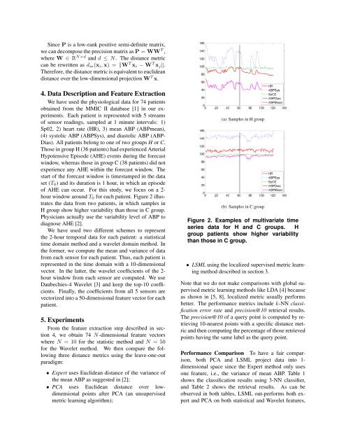
Since P is a low-rank positive semi-definite matrix, we can decompose the precision matrix as P = WW T , where W ∈ R N×d and d ≤ N. The distance metric can be rewritten as d m (x i , x) = ‖W T x i − W T x j ‖. Therefore, the distance metric is equivalent to euclidean distance over the low-dimensional projection W T x. 4. Data Description and Feature Extraction We have used the physiological data for 74 patients obtained from the MMIC II database [1] in our experiments. Each patient is represented with 5 streams of sensor readings, sampled at 1 minute intervals: 1) Sp02, 2) heart rate (HR), 3) mean ABP (ABPmean), (4) systolic ABP (ABPSys), and diastolic ABP (ABP- Dias). All patients belong to one of two groups H or C. Those in group H (36 patients) had experienced Arterial Hypotensive Episode (AHE) events during the forecast window, whereas those in group C (38 patients) did not experience any AHE within the forecast window. The start of the forecast window is timestamped in the data set (T 0 ) and its duration is 1 hour, in which an episode of AHE can occur. For this study, we focus on a 2- hour window around T 0 for each patient. Figure 2 illustrates the data from two patients, in which samples in H group show higher variability than those in C group. Physicians actually use the variability level of ABP to diagnose AHE [2]. We have used two different schemes to represent the 2-hour temporal data for each patient: a statistical time domain method and a wavelet domain method. In the former, we compute the mean and variance of data from each sensor for each patient. Thus, each patient is represented in the time domain with a 10-dimensional vector. In the latter, the wavelet coefficients of the 2- hour window from each sensor are computed. We use Daubechies-4 Wavelet [3] and keep the top-10 coefficients. Finally, the coefficients from all 5 sensors are vectorized into a 50-dimensional feature vector for each patient. 5. Experiments From the feature extraction step described in section 4, we obtain 74 N-dimensional feature vectors where N = 10 for the statistic method and N = 50 for the Wavelet method. We then compare the following three distance metrics using the leave-one-out paradigm: • Expert uses Euclidean distance of the variance of the mean ABP as suggested in [2]; • PCA uses Euclidean distance over lowdimensional points after PCA (an unsupervised metric learning algorithm); (a) Samples in H group (b) Samples in C group Figure 2. Examples of multivariate time series data for H and C groups. H group patients show higher variability than those in C group. • LSML using the localized supervised metric learning method described in section 3. Note that we do not make comparisons with global supervised metric learning methods like LDA [4] because as shown in [5, 8], localized metric usually performs better. The performance metrics include k-NN classification error rate and precision@10 retrieval results. The precision@10 of a query point is computed by retrieving 10-nearest points with a specific distance metric and then computing the percentage of those retrieved points having the same label as the query point. Performance Comparison To have a fair comparison, both PCA and LSML project data into 1- dimensional space since the Expert method only uses one feature, i.e., the variance of mean ABP. Table 1 shows the classification results using 3-NN classifier, and Table 2 shows the retrieval results. As can be observed in both tables, LSML out-performs both expert and PCA on both statistical and Wavelet features,
Page 1: Localized

Localized Supervised Metric Learning on ... - Researcher - IBM

You also want an ePaper? Increase the reach of your titles

Delete template?

Save as template?