Introduction to RF and Wireless
Introduction to RF and Wireless
Introduction to RF and Wireless

Create successful ePaper yourself
Turn your PDF publications into a flip-book with our unique Google optimized e-Paper software.
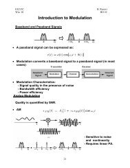
EE215C<br />
B. Razavi<br />
Win. 10 HO #2<br />
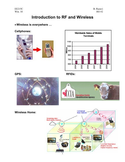
<strong>Introduction</strong> <strong>to</strong> <strong>RF</strong> <strong>and</strong> <strong>Wireless</strong><br />
• <strong>Wireless</strong> is everywhere …<br />
Cellphones:<br />
Worldwide Sales of Mobile<br />
Terminals<br />
1100<br />
1000<br />
900<br />
800<br />
700<br />
600<br />
2004<br />
2005<br />
2006<br />
2007<br />
2008<br />
Million<br />
2009<br />
GPS:<br />
<strong>RF</strong>IDs:<br />
<strong>Wireless</strong> Home:<br />
1
EE215C<br />
B. Razavi<br />
Win. 10 HO #2<br />
• <strong>Wireless</strong> design is challenging …<br />
- Draws upon many fields:<br />
- Competi<strong>to</strong>rs must push for: cost,<br />
talk time, sensitivity, functions, size,<br />
weight, …<br />
• <strong>Wireless</strong> has come a long way …<br />
[A. Behzad et al,<br />
ISSCC07]<br />
2x2 802.11a/b/g/n<br />
(18 mm 2 )<br />
2
EE215C<br />
B. Razavi<br />
Win. 10 HO #2<br />
Nonlinearity <strong>and</strong> Dis<strong>to</strong>rtion<br />
Linearity <strong>and</strong> Time Variance<br />
- A system is linear if it satisfies the superposition principle:<br />
- A system is time-variant if<br />
Example:<br />
If the switch turns on at the zero crossings of Vin1, is the system<br />
nonlinear or time-variant?<br />
- A linear system can generate frequency components that do not exist<br />
in the input:<br />
Graphically:<br />
3
EE215C<br />
B. Razavi<br />
Win. 10 HO #2<br />
Classes of Systems<br />
- Memoryless vs. Dynamic Systems: A memoryless (“static”) system<br />
produces an instantaneous output, i.e., the output does not depend on<br />
past values:<br />
A dynamic system produces an output that may depend on past<br />
values. A linear dynamic system satisfies the convolution integral:<br />
- For a static, nonlinear system, we can approximate the input/output<br />
relationship by a polynomial:<br />
Most types of nonlinearity<br />
encountered in practice are<br />
“compressive:<br />
- For a dynamic, nonlinear system, one may need <strong>to</strong> resort <strong>to</strong> Volterra<br />
series or “harmonic balance” techniques.<br />
Example:<br />
4
EE215C<br />
B. Razavi<br />
Win. 10 HO #2<br />
Effects of Nonlinearity<br />
Nonlinearity introduces “harmonic dis<strong>to</strong>rtion,” “gain compression,”<br />
“desensitization,” “intermodulation,” etc.<br />
• Harmonic Dis<strong>to</strong>rtion<br />
If a sinusoid is applied <strong>to</strong> a nonlinear time-invariant system, the output<br />
contains components that are integer multiples of the input frequency:<br />
If<br />
then<br />
- With “odd symmetry,” even harmonics are absent.<br />
- Amplitude of nth-order harmonic is roughly proportional <strong>to</strong> A n .<br />
-<br />
• Gain Compression<br />
In compressive systems, the small-signal gain (slope of the charac.) falls<br />
at high input levels. This is quantified by the “1-dB compression point:”<br />
• Desensitization <strong>and</strong> Blocking<br />
If a small signal is accompanied with a large interferer, then:<br />
5
EE215C<br />
B. Razavi<br />
Win. 10 HO #2<br />
The interferer is sometimes called a “blocker.”<br />
Example:<br />
• Intermodulation<br />
Suppose two interferers are applied <strong>to</strong> a nonlinear system (“two-<strong>to</strong>ne<br />
test”):<br />
We therefore have these “intermodulation” (IM) components:<br />
Which ones are troublesome?<br />
6
EE215C<br />
B. Razavi<br />
Win. 10 HO #2<br />
- “Third Intercept Point” (IP3): Two <strong>to</strong>nes with equal amplitudes are<br />
applied:<br />
Thus, IIP3 is obtained as:<br />
- Shortcut Method:<br />
- Relationship between IP3 <strong>and</strong> P1dB:<br />
Typical receiver IP3 is around -10 dBm.<br />
7
EE215C<br />
B. Razavi<br />
Win. 10 HO #2<br />
• Cascaded Nonlinear Stages<br />
Another perspective:<br />
8
EE215C<br />
B. Razavi<br />
Win. 10 HO #2<br />
EE101 Concepts<br />
• Definitions of Q<br />
For a second-order tank:<br />
• Conjugate Matching<br />
Do we want <strong>to</strong> have conjugate matching<br />
here?<br />
• dB’s <strong>and</strong> dBm’s<br />
dB is used for dimensionless quantities <strong>to</strong> make them algebraically<br />
manageable:<br />
- Voltage Gain: Vout/Vin in dB 20log (Vout/Vin)<br />
- Power Gain: Pout/Pin in dB 10log (Pout/Pin)<br />
Are the voltage gain <strong>and</strong> power gain equal if expressed in dB?<br />
9
EE215C<br />
B. Razavi<br />
Win. 10 HO #2<br />
dBm is used for power quantities is a 50-ohm matched system:<br />
Power P1 in dBm = 10 log (P1/ 1mW)<br />
What do we do in on-50-ohm systems?<br />
- A 50-ohm signal source delivers the specified power only if it is<br />
terminated in<strong>to</strong> a 50-ohm load.<br />
• Other Basics<br />
- Fourier transform of sine <strong>and</strong> cosine<br />
- Sifting property of impulses<br />
- Trig. Identities: cos a +/- cos b, cos a cos b, cos (a+b), cos 2 a,<br />
cos 3 a<br />
10
EE215C<br />
B. Razavi<br />
Win. 10 HO #2<br />
Noise in <strong>RF</strong> Design<br />
What is Noise?<br />
Noise is a r<strong>and</strong>om process. Since the instantaneous noise amplitude is<br />
not known, we resort <strong>to</strong> “statistical” models, i.e., some properties that<br />
can be predicted.<br />
Average Power<br />
Larger fluctuations mean that<br />
the noise is “stronger.”<br />
Normalized average power:<br />
Statistical Characterization<br />
• Frequency-Domain Behavior<br />
For r<strong>and</strong>om signals, the concept of Fourier transform cannot be directly<br />
applied. But we still know that men carry less high-frequency<br />
components in their voice than women do.<br />
11
EE215C<br />
B. Razavi<br />
Win. 10 HO #2<br />
We define the “power spectral density” (PSD) (also called the<br />
“spectrum”) as:<br />
The PSD thus indicates how<br />
much power the signal carries<br />
in a small b<strong>and</strong>width around<br />
each frequency.<br />
Example: Thermal Noise Voltage of a<br />
Resis<strong>to</strong>r<br />
A flat spectrum is called “white.”<br />
• Is the <strong>to</strong>tal noise power infinite?<br />
• What is the <strong>to</strong>tal noise power in 1 Hz?<br />
• What is the unit of S(f)?<br />
Important Theorem<br />
12
EE215C<br />
B. Razavi<br />
Win. 10 HO #2<br />
For mathematical convenience, we may “fold” the spectrum as shown<br />
here:<br />
Example<br />
Calculate the <strong>to</strong>tal rms noise at the output of this circuit.<br />
• The PDF <strong>and</strong> PSD generally bear no relationship:<br />
Thermal Noise: Gaussian, white<br />
“Flicker” Noise: Gaussian, not white<br />
Not<br />
e:<br />
Correlated <strong>and</strong> Uncorrelated Sources<br />
Can we use superposition for noise components?<br />
13
EE215C<br />
B. Razavi<br />
Win. 10 HO #2<br />
Types of Noise<br />
1. Thermal Noise<br />
R<strong>and</strong>om movement of charge carriers in a resis<strong>to</strong>r causes fluctuations<br />
in the current. The PDF is Gaussian because there are so many carriers.<br />
The PSD is given by:<br />
Note that the polarity of the voltage source is arbitrary.<br />
• Example: A 50-Ώ resis<strong>to</strong>r at room temperature exhibits an RMS noise<br />
voltage of .<br />
If this resis<strong>to</strong>r is used in a system with 1-MHz b<strong>and</strong>width, then it<br />
contributes a <strong>to</strong>tal rms voltage of .<br />
The ohmic resistances in transis<strong>to</strong>rs<br />
contribute thermal noise:<br />
Example:<br />
The ohmic sections also contribute thermal<br />
noise:<br />
14
EE215C<br />
B. Razavi<br />
Win. 10 HO #2<br />
In a well-designed layout, only the channel thermal (<strong>and</strong> flicker) noise<br />
may be dominant:<br />
2. Shot Noise<br />
If carriers cross a potential barrier, then the overall current actually<br />
consists of a large number of r<strong>and</strong>om current pulses. . The r<strong>and</strong>om<br />
component of the current is called “shot noise” <strong>and</strong> given by:<br />
Note that shot noise does not depend on the temperature.<br />
Shot noise occurs in pn-junction diodes, bipolar transis<strong>to</strong>rs, <strong>and</strong><br />
MOSFETs operating in subthreshold region.<br />
3. Flicker (1/f) Noise<br />
In MOSFETs, the extra<br />
energy states at the<br />
interface between silicon<br />
<strong>and</strong> oxide trap <strong>and</strong> release<br />
carriers r<strong>and</strong>omly <strong>and</strong> at<br />
different rates. The noise in<br />
spectrum referred <strong>to</strong> the gate is given by:<br />
Where k is a constant <strong>and</strong> its value heavily<br />
depends on how “clean” the process is. We often<br />
characterize the seriousness of 1/f noise by<br />
considering the 1/f “corner” frequency.<br />
15
EE215C<br />
B. Razavi<br />
Win. 10 HO #2<br />
Representation of Noise in Circuits<br />
• Input-Referred Noise<br />
Input-referred noise is the noise voltage or current that, when applied <strong>to</strong><br />
the input of the noiseless circuit, generates the same output noise as the<br />
actual circuit does.<br />
In general, we need both a voltage<br />
source <strong>and</strong> a current source at the<br />
input <strong>to</strong> model the circuit noise:<br />
If the source impedance is high with respect <strong>to</strong> the input impedance of<br />
the circuit, then both must be considered.<br />
- How do we calculate the input-referred noise?<br />
Important Note: These two components may be correlated in many<br />
cases.<br />
16
EE215C<br />
B. Razavi<br />
Win. 10 HO #2<br />
Example<br />
• Noise Figure<br />
At high frequencies, it becomes difficult <strong>to</strong> measure the input-referred<br />
noise voltage <strong>and</strong> current <strong>and</strong> their correlation. We therefore seek a<br />
single metric that represents the noise behavior:<br />
Notes:<br />
- NF measures how much the SNR degrades as the signal passes thru<br />
the system.<br />
- If the input has no noise, NF is meaningless.<br />
Calculation of NF:<br />
NF<br />
17
EE215C<br />
B. Razavi<br />
Win. 10 HO #2<br />
Example<br />
Typical LNAs achieve a noise figure of about 2dB.<br />
• NF of Cascaded Stages<br />
The <strong>to</strong>tal voltage gain is equal <strong>to</strong>:<br />
Thus,<br />
Not much intuition here. In traditional microwave design, all interfaces<br />
are matched <strong>to</strong> 50 ohms, <strong>and</strong><br />
18
EE215C<br />
B. Razavi<br />
Win. 10 HO #2<br />
More generally, the NF can be expressed in terms of the “available<br />
power gain,” Ap, defined as the available power at the output divided by<br />
the available source power:<br />
This is called Friis’ Equation. Note that each NF must be calculated with<br />
respect <strong>to</strong> the output impedance of the preceding stage.<br />
But how do we do this for this cascade:<br />
• NF of Lossy Circuits<br />
If the available power loss L is defined as the available source power<br />
divided by the available output power, then NF = L.<br />
For a cascade:<br />
19
EE215C<br />
B. Razavi<br />
Win. 10 HO #2<br />
Sensitivity <strong>and</strong> Dynamic Range<br />
- Sensitivity is defined as the minimum signal level that can be detected<br />
with “acceptable” quality. With digital modulation schemes, the quality<br />
is measured by the “bit error rate” (BER).<br />
The available noise power for a resis<strong>to</strong>r is given by:<br />
Thus,<br />
Note that the sensitivity is a function of b<strong>and</strong>width <strong>and</strong> hence the bit<br />
rate. For example,<br />
GSM:<br />
11a:<br />
- Spurious-free dynamic range (SFDR) in <strong>RF</strong> design is defined as the<br />
maximum level in a two-<strong>to</strong>ne test that produces an IM3 product equal <strong>to</strong><br />
the noise floor divided by the sensitivity.<br />
Since<br />
we have<br />
For example, NF = 9 dB, IP3=-15 dBm, B= 200 kHz, SNR min =12 dB<br />
SFDR=53 dB.<br />
20