IIT-JEE 2010 - Career Point

X
O
4
C
A
8 F
B
10.4
14
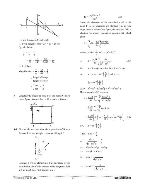
F is at a distance 2.4 cm from C.
∴ Focal length of lens = 2.4 × 10 = 24 cm
By calculation
1 1 1 = –
f v u
1 1
= – 60 − 40
∴ f = 24 cm
100 1
= = 2400 24
v 60 3
Magnification = = = u 40 2
=
=
length of image
length of object
3 mm
2 mm
= 2
3
5. Calculate the magnetic field B at the point P shown
in the figure. Assume that i = 10 A and a = 8.0 cm.
B a/4
a
4
i
A
P
i
Sol. First of all, we determine the expression of B at a
distance R from a straight conductor of length l.
x
x 2
x 1
φ
dx
i
R
Consider a typical element dx. The magnitude of the
contribution dB of this element to the magnetic field
at P as found from Biot-Savart's law is
r
C
i
D
I
X
µ 0idxsin
θ
dB =
...(i)
2
4πr
Since, the direction of the contribution dB at the
point P for all elements are identical viz, at right
angle into the plane of the figure, the resultant field is
obtained by simply integration equation (i), which
gives
x
B =
∫ 2 µ 0i
dB =
4π
x1
x 2
∫
x1
sin θdx
where, sin θ = r
R and r = (x 2 + R 2 ) 1/2
µ 0iR
∴ B =
4π
x2
r
∫
+
x1
2
dx
2 2
( x R )
3/ 2
Let x = R tan φ, such that dx = R sec 2 φ dφ
At x = x 1 φ 1 = tan –1 ⎛ x ⎞
⎜ 1
⎟ and x = x 2 ,
⎝ R ⎠
x 2
φ 2 = tan –1 ⎛ ⎞
⎜ ⎟
⎝ R ⎠
Also, x 2 + R 2 = R 2 tan 2 φ + R 2 = R 2 sec 2 φ
Hence, equation (ii) becomes
B =
µ 0iR
4π
∫ − 1 x
tan
2
R
−1
x
tan
1
R
µ tan
=
∫ −
0iR
−
4π
tan
1 x2
R
1 x1
R
R sec
R
3
sec
2
2
φ
φ
cosφ
dφ
...(ii)
µ 0 iR ⎡ ⎛ −1
x 2 ⎞ ⎛ −1
x1
⎞⎤
= ⎢sin⎜
tan ⎟ − sin⎜
tan ⎟⎥ ...(iii)
4π
⎣ ⎝ R ⎠ ⎝ R ⎠ ⎦
Let, z = tan –1 ⎛ x ⎞
⎜ ⎟ ,
⎝ R ⎠
x
Thus, tan z = R
⇒
sin z
1−
sin
2
z
= R
x
⇒ R 2 sin 2 z = x 2 (1 – sin 2 z)
⇒ sin 2 z(R 2 + x 2 ) = x 2
⇒ sin z =
x
2
x
+ R
⎛
⇒ z = sin –1 ⎟ ⎟ ⎞
⎜ x
⎜
⎝ x 2 + R
2 ⎠
2
XtraEdge for IIT-JEE 24 DECEMBER 2009