Mathematical Models for Nano Science - Politecnico di Milano

Mathematical Models
for Nano Science
July 4 th 2011
Matteo Porro
Center for Nano Science and Technology of IIT@PoliMi
Dipartimento di Matematica ”Francesco Brioschi”
Politecnico di Milano

Introducing myself
Education
• 2004 - 2008
B.Sc. in Mathematical Engineering at Politecnico di Milano
thesis: Parametric analysis of the dynamics of a rowing boat
• 2008 - 2010
M.Sc. in Mathematical Engineering at Politecnico di Milano
thesis: Third generation solar cells: modeling and simulation
Current position
• 2011
Fellow internship at CNST of IIT@PoliMi
Future plans (???)
• 2011 -
Ph.D. in Mathematical Models and Methods in Material Science
at Politecnico di Milano

Math Research Group
Prof. Riccardo Sacco
• M.Sc. in Electronic Engineering and Ph.D. in Applied
Mathematics
Prof. Maurizio Verri
• M.Sc. in Physics
Carlo de Falco, Ph.D.
• M.Sc. in Electronic Engineering and Ph.D. in Mathematics
and Statistics for Computational Science
Marco Carnini, Ph.D.
• M.Sc. in Physics and Ph.D. in Mathematical Engineering

Summary
Past activity
• Bulk heterojunction organic solar cell model
• Bilayer organic solar cell model
Present and future activity
• SuperC model
• Artificial retina model

Bulk Heterojunction solar cells
light
current
at contacts
absorbption
radiative
recombination
drift / diffusion
bulk
excitons
diffusion
bulk
free carriers
interface
excitons
partial
dissociation
geminate
recombination pairs
drift / diffusion
recombination
interface
free carriers
recombination to
triplet excitons
dissociation
L
Γ N
Γ C
hν
Ω
Γ A
Γ N
Assumptions
• Homogeneity. Blend as a single material
with averaged properties
• Immediate transition exciton → charge
transfer state
• Einstein relation
Unknowns: X , n, p and ϕ

Model equations - 1
• Excited state
equation
{ ∂X
∂t = G − k recX − k diss X + γnp in Ω
X (x, 0) = X 0 (x) in Ω.
• No diffusion → ODE → no need for boundary conditions
• Generation term G(x, t): constant, Beer-Lambert
• Dissociation rate constant k diss (E) according to Onsager theory
• Langevin bimolecular recombination γnp
• Electron
equation
⎧
∂n
∂t − 1 q div J n = k diss X − γnp in Ω
⎪⎨
J n = qD n ∇n − qµ n n∇ϕ in Ω
1
γ n
q J n · ν = β n − α n n on Γ A ∪ Γ C
⎪⎩
n(x, 0) = n 0 (x) in Ω.
• Drift-Diffusion model • Scott-Malliaras boundary conditions
• Simplified Poole-Frenkel model for mobility µ(E)

• Hole
equation
Model equations - 2
⎧
∂n
∂t + 1 q div J p = k diss X − γnp in Ω
⎪⎨
J p = −qD p ∇p − qµ p p∇ϕ in Ω
1
−γ p
q J p · ν = β p − α p p on Γ A ∪ Γ C
⎪⎩
p(x, 0) = p 0 (x) in Ω.
• Similar to electron equation. Just some differences in the signs
• Poisson
equation
⎧
⎪⎨
( )
−div ε 0 ε r ∇ϕ = q ( p − n ) in Ω
ϕ = V appl − V bi
⎪⎩
ϕ = 0
on Γ A
on Γ C
• Applied and bias potential → Dirichlet boundary conditions
• Electric field E = −∇ϕ

Numerical Approach
Rothe method
• Fully coupled system
• Strongly nonlinear equations
• Time discretization with Runge-Kutta methods
• Linearization of the problems
• Spatial discretization
Functional iteration algorithms
• Newton method: faster convergence but less robust.
• Gummel map: staggered algorithm, (possibly) slower but
robust. Also useful as a solution map for the analysis of
existence/uniqueness.

Spatial discretization
Triangulation of the domain
• Structured
• Unstructured
Methods
• Finite difference • Finite element • Finite volume
Possibly arising problems
• Instability/numerical oscillations
• Flux conservation issues
• Undesired negative values

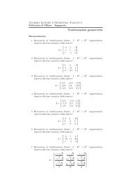
1D examples
Dominant transport
{
− 1 ε u′′ + u ′ = 1 x ∈ (0, 1)
u(0) = 0, u(1) = 0
• ε = 10 2
Dominant reaction
{
− 1 ε u′′ + u = 1 x ∈ (0, 1)
u(0) = 0, u(1) = 0
• ε = 10 4
1.6
1.4
1.2
1
Exact solution
Numerical solution n=10
Numerical solution n=20
1.2
1
0.8
u(x)
0.8
u(x)
0.6
0.6
0.4
0.2
0
0 0.2 0.4 0.6 0.8 1
x
0.4
0.2
0
Exact solution
Numerical solution n=10
Numerical solution n=20
0 0.2 0.4 0.6 0.8 1
x
• Many points for stability, even more in 2D or 3D
• Solution: stabilization techniques and ad-hoc schemes

Numerical results - 1
• Ideal BHJ solar cell
• Short circuit condition (V appl = 0 V)
• Same mobility for holes and electrons
• Transient simulation in (0, 10 µs)
• Low illumination
G = 4.3 · 10 26 m −3 s −1
• High illumination
G = 4.3 · 10 30 m −3 s −1
4 x 1019 Position [nm]
2.5 x 1023 Position [nm]
Electron density [m −3 ]
3.5
3
2.5
2
1.5
1
0.5
0
0 10 20 30 40 50 60 70
Electron density [m −3 ]
2
1.5
1
0.5
0
0 10 20 30 40 50 60 70
C. de Falco & al. 2010

Numerical results - 2
• Photodetector fabricated in DEI labs
• BHJ of squaraine dyes and PCBM (ratio 1:3)
• Thickness 220 nm, area 4 mm 2 , I = 6.3 Wm −2 , λ = 700 nm
0
x10 -7
• With light
measured data
simulation results
• Dark
Current [A]
-5
-10
-15
0 0.1 0.2 0.3 0.4 0.5
Applied bias [V]
M. Binda & al. 2009
C. de Falco & al. 2010

Bilayer solar cells
light
current
at contacts
absorbption
radiative
recombination
drift / diffusion
bulk
excitons
diffusion
bulk
free carriers
interface
excitons
partial
dissociation
geminate
recombination pairs
drift / diffusion
recombination
interface
free carriers
recombination to
triplet excitons
dissociation
2H
Ω n
Γ C
hν
Ω H
Γ N
Assumptions
• Depletion of electrons in Ω p and of
holes in Ω n
Ω p
• Dissociation area Ω H
• Einstein relation
Γ A
Unknowns: X , P, n, p and ϕ

Model equations - 1
• Exciton
equation
⎧
∂X
∂t + div J X = G − X τ X
⎪⎨
∂X
∂t + div J X = G − X −
X + ηk rec P
τ X τ diss
J X = −D X ∇X
in Ω n ∪ Ω p
in Ω H
in Ω
X = 0
on Γ C ∪ Γ A
⎪⎩
X (x, 0) = X 0 (x) in Ω.
• Excitons have null net charge → Only diffusion (Fick law)
• Generation term G(x, t): constant, Beer-Lambert
• Exciton lifetime τ X , geminate pair formation time τ diss
• Geminate pair recombination rate constant k rec and triplet
exciton fraction η
• X and J X are continuous in Ω

Model equations - 2
• Geminate pair
equation
⎧
∂P
⎪⎨ ∂t = X − (k diss + k rec )P + γnp in Ω H
τ diss
P = 0
in Ω n ∪ Ω p
⎪⎩
P(x, 0) = P 0 (x) in Ω.
• No diffusion → ODE → no need for boundary conditions
• Modified dissociation rate constant k diss (E)
• Langevin bimolecular recombination γnp
• Electron
equation
(Hole equation
is analogous)
⎧
∂n
∂t − 1 q div J n = 0
∂n
⎪⎨ ∂t − 1 q div J n = k diss P − γnp
J n = qD n ∇n − qµ n n∇ϕ
n = 0
in Ω n
in Ω H
in Ω n ∪ Ω H
in Ω p
n = n C
on Γ C
⎪⎩
n(x, 0) = n 0 (x) in Ω.

Model equations - 3
• Poisson
equation
⎧ ( )
−div ε∇ϕ = −qn in Ω n
( )
−div ε∇ϕ = +q ( p − n ) in Ω ⎪⎨
H
( )
−div ε∇ϕ = +qp in Ω p
ϕ = V appl − V bi
⎪⎩
ϕ = 0
on Γ A
on Γ C
• Applied and bias potential → Dirichlet boundary conditions
• The dielectric constant ε may vary in the materials
• The electric potential ϕ and the normal component of the
electric displacement field −ε∇ϕ · ν are continuous

Interface lumping - 1
• Device thickness ≫ active layer thickness
(∼ 10 2 /∼ 10 0 nm)
• Still a certain number of nodes in Ω H is
needed
Idea
• Neglect the thickness of the active layer
• Assume the phenomena to occur just on
the mathematical interface Γ
• Many nodes
Γ C
Γ N
Ω n
Γ
hν
Ω p
Γ N
New computational
domain
• Less nodes
• Same definition
Γ A

Interface lumping - 2
Lumping procedure
• Integrate the equations in Ω H and let active layer thickness
H → 0
• P becomes surface density
• Volumetric terms in the equations → flux interface conditions
[[X ]] = 0,
[[J X · ν]] = ηk rec P − 2H
τ diss
X
on Γ
∂P
∂t = 2H
τ diss
X − (k diss + k rec ) P + 2Hγnp on Γ.
1
q J n · ν = 1 q J p · ν = −k diss P + 2Hγnp
[[A]] is the jump of A across Γ
[[ϕ]] = [[ε∇ϕ · ν]] = 0
on Γ
on Γ

Numerical results - 1
Ω p
Γ
Γ C
Ω n
• Ideal morphology of
nanostructured
polymers
• Cell thickness 150 nm,
nanorods 79 × 55 nm
Current Density [mA m −2 ]
100
80
60
40
20
Γ A
• V bi = 0.6 V 0
0 0.2 0.4 0.6 0.8 1
Applied Potential [V]
Open Circuit Voltage [V]
1.1
1
0.9
0.8
0.7
10 20 10 21 10 22 10 23 10 24 10 25 10 26
Exciton Generation Rate [m −3 s −1 ]
de Falco & al. 2011
Short Circuit Current Density [mA m −2 ]
10 0
10 −2
10 −4
10 −6
10 20 10 22 10 24 10 26 10 28 10 30
10 2 Exciton Generation Rate [m −3 s −1 ]

Numerical results - 2
Short circuit (V appl = 0 V) Open circuit (V appl = 0.9 V)
de Falco & al. 2011

Numerical results - 3
• Very complex morphology
• Remarkable reduction of
computational cost
de Falco & al. 2011
Current Density [mA m −2 ]
60
50
40
30
20
10
0
0 0.2 0.4 0.6 0.8 1
Applied Potential [V]

Conclusions and future work
Conclusions
• Development of a PDE/ODE model for organic solar
cells
• Validation on real devices and numerical results from
literature
Future work
• Implementation of a 3D version of the model
• Inclusion of solar radiation spectrum and of material
absorption spectrum
• Further validation on experimental data, possibly with
different devices
• More accurate models for physical parameters

Activity at CNST - SuperC
• Photoactivated capacitor
• Structure similar to that of
a solar cell
• Possibility of stacking
multiple layers with
different materials
Au electrode
dielectric
H2PC/CuPC
PTCBI/C60
dielectric
H2PC/CuPC
d d d a h
PTCBI/C60
dielectric
nd d + nd a + (n + 1)h
dielectric
H2PC/CuPC
PTCBI/C60
dielectric
ITO electrode
Vc(t)
C
- - - - - - - -
+ + + +
+ + + +
+
+
+
+
+ +
- - - - - - - -
+ +
Vp(t)
i(t)
• Included blackbody
radiation with material
absorption spectra
• Same model as organic solar
cells with modifications for
zero outward current flux
• Possibly back to volumetric
model (L dev ≃ H)
R

Activity at CNST - Artificial Retina
Structure
• Photoactive
polymer layer
• Electrolyte
• Neuronal cell
V m
V b
C i
R s
R i
Polymer
ITO
Proposed model
• Bulk/bilayer solar
cell model
• Poisson-Nernst-
Planck
model
• Hodgkin–Huxley
model
Major issues
Substrate
• Rates of electrochemical reactions
strongly dependent on local potential
and concentrations
• Treatment of ionic layers in the liquid
phase close to the interfaces